插值法——lagrange插值

　　1.插值函数

%%n次插值多项式
%%X是插值节点，n是插值多项式次数，若已知函数表达式则attribute为0，未知函数表达式但已知函数值时为1
function IPn = Interpolation_polynomials_of_degree_n(X,Y,precision,attribute)
global MAX;global m;global n;global i;
X = sort(X);
[m,n] = size(X);MAX = max([m,n]);error = [];
if attribute == 0
    F = ones(1,MAX);
    for i = 1:MAX
        F(i) = subs(Y,X(i));
    end
    sum = 0;
    for i = 1:MAX
        sum = sum+F(i)*Interpolation_basis_fun(X,i-1);
    end
    IPn = vpa(collect(sum),4);
    for i = 1:MAX
        error(i) = abs(F(i)-subs(sum,X(i)));
    end
    
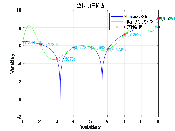
    %%作图
    h=figure;
    set(h,'color','w');
    t = min(X):(max(X)-min(X))/precision:max(X);
    Yreal = subs(Y,t);
    T = subs(sum,t);
    plot(t,Yreal,'b',t,T,'g',X,F,'r*');
    grid on
    title('拉格朗日插值');
    xlabel('Variable x');
    ylabel('Variable y');
    legend('Yreal:真实图像','T:拟合多项式图像','F:实际数据');
    
    %%显示坐标
    for i = 1:MAX
        text(X(i),F(i),['(',num2str(X(i)),',',num2str(F(i)),')'],'color',[0.02 0.79 0.99]);
    end
     disp('误差值为');error

elseif attribute == 1
    sum = 0;
    for i = 1:MAX
        sum = sum+Y(i)*Interpolation_basis_fun(X,i-1);
    end
    IPn = vpa(collect(sum),4);
    
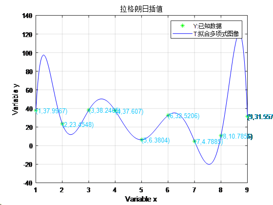
    h=figure;
    set(h,'color','w');
    t = min(X):(max(X)-min(X))/precision:max(X);
    T = subs(sum,t);
    plot(X,Y,'g*',t,T,'b');
    grid on
    title('拉格朗日插值');
    xlabel('Variable x');
    ylabel('Variable y');
    legend('Y:已知数据','T:拟合多项式图像');
    for i = 1:MAX
        text(X(i),Y(i),['(',num2str(X(i)),',',num2str(Y(i)),')'],'color',[0.02 0.79 0.99]);
    end
end
end

　　2.插值基函数

%%插值基函数
function IBF = Interpolation_basis_fun(X,k)
[m,n] = size(X);MAX = max([m,n]);
X = sort(X);
mult_x = 1;mult_v = 1;
for i = 1:MAX
    syms x;
    if i ~= k+1
        mult_v = mult_v*(X(k+1)-X(i));
        mult_x = mult_x*(x-X(i));
    end
end
IBF = mult_x/mult_v;
end

　　3.插值余项与误差界

%%插值余项与误差限（仅能计算已知的函数表达式下的余项）
function MI = More_than_the_interpolation(X,f,xi,precision)
X = sort(X);
a = min(X);b = max(X);
disp('xi应在以下区间中：');
[a,b]
[m,n] = size(X);MAX = max([m,n]);
Df = diff(f,MAX);Df_value = subs(Df,xi);
MI = vpa(collect(Df_value*omiga(X)/factorial(MAX)),4);

%%误差限
Df_max = max(subs(Df,X));
R_x = vpa(collect(Df_max*abs(omiga(X))/factorial(MAX)),4);
disp('误差上限为：');
R_x

%%作图区
t = a:(b-a)/precision:b;
T1 = subs(R_x,t);
T2 = subs(MI,t);
h=figure;
set(h,'color','w');
plot(t,T1,'r--',t,T2,'g');
    grid on
    title('误差图像');
    xlabel('Variable x');
    ylabel('Variable y');
    legend('T1:误差上限','T2:指定误差限');

    function fac = Factorial(n)
        if n == 0
            fac = 1;
        else
            fac = Factorial(n-1)*n;
        end
    end
end

　　4.连乘多项式

function ox = omiga(X)
[m,n] = size(X);MAX = max([m,n]);
syms x;
mult = 1;
for i = 1:MAX
    mult = mult*(x-X(i));
end
ox=mult;
end

　　5.例子

clear all
clc
precision=500;
X=1:1:9;
R1=reshape(rand(9),1,9^2);
R2=reshape(rand(18),1,18^2);
R=zeros(1,9);
for i=1:9
    R(i)=R1(9*i)*R2(18*i)*100;
end

%%已知函数
disp('已知函数的表达式');
syms x;
f=x*exp(-x^2)+log(abs(exp(x)+precision*sin(x)));
Interpolation_polynomials_of_degree_n(X,f,precision,0)

%%已知函数数值
disp('已知函数值');
Interpolation_polynomials_of_degree_n(X,R,precision,1)

　　结果

已知函数的表达式
误差值为
error =
     0     0     0     0     0     0     0     0     0
ans =
1.621e-5*x^8 + 0.002542*x^7 - 0.1033*x^6 + 1.566*x^5 - 12.15*x^4 + 52.22*x^3 - 122.5*x^2 + 141.6*x - 54.27
已知函数值
ans =
- 0.06151*x^8 + 2.428*x^7 - 40.08*x^6 + 359.3*x^5 - 1899.0*x^4 + 6000.0*x^3 - 10950.0*x^2 + 10420.0*x - 3849.0

　　图像如下