原文:
http://blog.sina.com.cn/s/blog_4ba16d110102vilj.html
https://blog.csdn.net/rainday0310/article/details/9130143
https://jingyan.baidu.com/article/e52e36151a862740c60c51e8.html
公式
=VLOOKUP(A2,列2!$A:$F,2,FALSE)
=VLOOKUP(A2,列2!$A:$F,COLUMN()-5,FALSE)
目的
列1 这个sheet

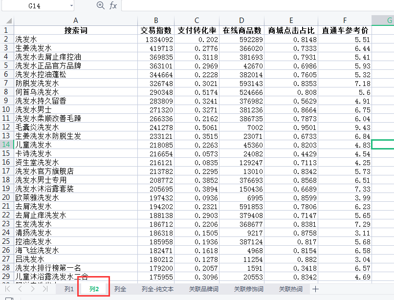
列2 这个sheet
目的
想通过 搜索词 这个列,来连接两个表
最终效果要是这个样子

所用到的公式
=VLOOKUP(A2,列2!$A:$F,2,FALSE)
=VLOOKUP(A2,列2!$A:$F,COLUMN()-5,FALSE)
公式中每个参数的意思
第一个参数A2指以A2单元格中数据作为查找的字符,指定查找的值
第二个参数Sheet2!$A:$B 是指在工作表 sheet2 中查找并引用查找结果的 A至B列,指定查找的范围
第三个参数是需要引用的数据所在的列号,因为需要引用username,在B列,即第2列
第四个参数为模糊查找开关,false为精确匹配,true为非精确
COLUMN():获取当前列