PointNet网络深度学习在点云处理上的先驱,这个团队又提出了PointNet++模型。以下是我学习之余的总结,一是理清自己的思路,二是于无意看到这篇博文的您一起学习。
一、PointNet的问题
一般提出新的模型,总是要分析原有模型的不足,是的。
由PointNet网络结构可以看出,网络只是把全部点拼接在一起,提取一个全局特征,很少考虑一个点的领域结构,而领域是一个十分重要的概念。
PointNet不捕获由度量空间点引起的局部结构,限制了它识别细粒度图案和泛化到复杂场景的能力,简单理解就是功能不强,实际应用效果一般。
二、PointNet++优点
1.一种分层的神经网络,在输入点集的嵌套分区上迭代使用PointNet。
2.利用度量空间的距离,能够利用上下文尺度的增长学习局部特征。
3.由于不同位置采集的点云数据的密度不一样,能够自适应地结合多尺度特征。
三、介绍
1.什么是分层的网络结构?
PointNet首先把点集划分为一些重叠的局部区域(划分方法稍后介绍),类似于CNNs,从小的局部区域捕获细粒度的局部结构来提取局部特征。之后局部特征被分组到更大的单元,迭代,已提取更高level的特征,这个过程不断重复,直到我们获取的整个输入点集的特征(特征提取方法稍后介绍)。
2.如何把点集分组?
把每一个分组考虑成基础欧几里得空间的一个Neighborhood ball。领域球的参数就是质心的位置和尺度。采样的算法是Farthest point sampling(FPS),最远点采样法优势是可以尽可能的覆盖空间中的所有点。,使用FPS采样到一些中心点,然后使用K nearest neighbor(KNN)或者Ball query算法分组。
3.FPS算法:
流程很简单,以点云第一个点,作为查询点,加入点集A,从剩余点中,取一个距离点集A最远的点,一直采样到目标数量N为止。
一个点P到到点集A距离的定义:
P点到A中距离最近的一个点的距离,(min(dis(P,A_1),...dis(P,A_n)))。
具体实现是存在计算优化。
- 时间复杂度:每次选一个点,需要计算 (n) 个距离;选 (k) 个点,时间复杂度可以认为是:(nk) ,由于 (n) 和 (n) 是常数关系,所以也可以认为是: (n^2) 。
- 空间复杂度:需要一个长度为 (n)的数组,来记录、更新每个点的距离值,所以复杂度为: (O(n))。
看一下FPS调用函数,输入是点集,输出是多组点。
def farthest_point_sample(npoint,inp):
    '''
input:
    int32
    batch_size * ndataset * 3   float32
returns:
    batch_size * npoint         int32
    '''
    return sampling_module.farthest_point_sample(inp, npoint)
4.KNN和Ball query
KNN是是查找一个固定个数的领域点。Ball query是操作区域半径范围内的全部点(上限为K)。
5.如何确定分组尺度
一个常见的问题是,输入点集在不同区域点的密度不同。CNN使用小的卷积核效果较好,但是PointNet++不一定,领域太小可能点的数量太少。
PointNet++利用多尺度实现模型的鲁棒性,同时在训练的时候采用dropout,网络能够自适应取得多尺度组合的特征。
5.如何学习局部特征?
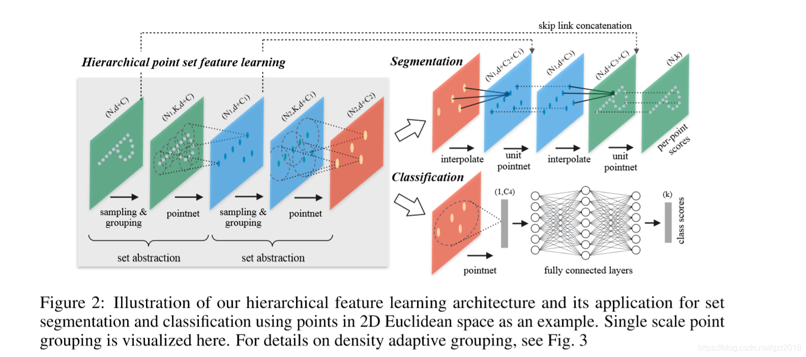
采样和分组都是为了特征学习,把一个领域球当作一个局部特征,使用一个小的PointNet提取特征,随着不同level的set abstraction(下面介绍),中心点个数不断减少,但是特征的维度越来越高。具体分类和分割网络模型如下。
四、模型构建方法
1.PointNet
PointNet是一个全局的函数拟合。缺乏不同规模上捕捉局部上下文的能力。所以PointNet采用分层特征学习框架。
2.分层网络的特征学习
分层网络结构由一些set abstraction层组成,每一层包含三个关键layers。一个set abstraction level把(N imes(d+C))矩阵为input,代表N个点,每个点d维坐标和C维特征。(N' imes(d+C'))矩阵为output,表示N'个子采样的点,每个点d维坐标和C维特征。
- Sampling layer :对输入点集采样,选出若干中心点,定义局部区域的质心,使用FPS。
- Grouping layer : 通过查找质心周围的“邻近”点来构建局部区域集,使用Ball query 算法找到半径范围内的全部点,上限为K。
- PointNet layer :使用小型PointNet将局部区域模式编码为特征向量,这一层的input为(N')个局部区域,数据大小为(N' imes K imes(d+C)),output是(N' imes(d+C')),字母意思应该很明确了。
对照图看一下采样和分组的代码,思路更加清晰:
def sample_and_group(npoint, radius, nsample, xyz, points, knn=False, use_xyz=True):
    '''
    Input:
        npoint: int32,关键点个数
        radius: float32
        nsample: int32,一分组点的个数
        xyz: (batch_size, ndataset, 3) TF tensor,ndataset表示一个size的总点数
        points: (batch_size, ndataset, channel) TF tensor, if None will just use xyz as points,可以理解成每个点特征信息
        knn: bool, if True use kNN instead of radius search
        use_xyz: bool, if True concat XYZ with local point features, otherwise just use point features
    Output:
        new_xyz: (batch_size, npoint, 3) TF tensor
        new_points: (batch_size, npoint, nsample, 3+channel) TF tensor
        idx: (batch_size, npoint, nsample) TF tensor, indices of local points as in ndataset points
        grouped_xyz: (batch_size, npoint, nsample, 3) TF tensor, normalized point XYZs,分好组的点
            (subtracted by seed point XYZ) in local regions
    '''
	#找到中心点 (new xyz),每个group的局部特征(new points),每个group对应的下标(idx)
    new_xyz = gather_point(xyz, farthest_point_sample(npoint, xyz)) # (batch_size, npoint, 3)
    if knn:
        _,idx = knn_point(nsample, xyz, new_xyz)
    else:
        idx, pts_cnt = query_ball_point(radius, nsample, xyz, new_xyz)
    grouped_xyz = group_point(xyz, idx) # (batch_size, npoint, nsample, 3)
    grouped_xyz -= tf.tile(tf.expand_dims(new_xyz, 2), [1,1,nsample,1]) # translation normalization
    if points is not None:
        # 把points按照上面分组的方法分组
        grouped_points = group_point(points, idx) # (batch_size, npoint, nsample, channel)
        if use_xyz:
            # concat操作,也就是论文中的d+C
            new_points = tf.concat([grouped_xyz, grouped_points], axis=-1) # (batch_size, npoint, nample, 3+channel)
        else:
            new_points = grouped_points
    else:
        new_points = grouped_xyz

    return new_xyz, new_points, idx, grouped_xyz
下面是set abstraction的代码,没有加入多尺度的特征提取:
def pointnet_sa_module(xyz, points, npoint, radius, nsample, mlp, mlp2, group_all, is_training, bn_decay, scope, bn=True, pooling='max', knn=False, use_xyz=True, use_nchw=False):
    ''' PointNet Set Abstraction (SA) Module
        Input:
            xyz: (batch_size, ndataset, 3) TF tensor,输入点集
            points: (batch_size, ndataset, channel) TF tensor,输入点集的特征
            npoint: int32 -- #points sampled in farthest point sampling
            radius: float32 -- search radius in local region
            nsample: int32 -- how many points in each local region
            mlp: list of int32 -- output size for MLP on each point
            mlp2: list of int32 -- output size for MLP on each region
            group_all: bool -- group all points into one PC if set true, OVERRIDE
                npoint, radius and nsample settings
            use_xyz: bool, if True concat XYZ with local point features, otherwise just use point features
            use_nchw: bool, if True, use NCHW data format for conv2d, which is usually faster than NHWC format
        Return:
            new_xyz: (batch_size, npoint, 3) TF tensor
            new_points: (batch_size, npoint, mlp[-1] or mlp2[-1]) TF tensor
            idx: (batch_size, npoint, nsample) int32 -- indices for local regions
    '''
    data_format = 'NCHW' if use_nchw else 'NHWC'
    with tf.variable_scope(scope) as sc:
        # Sample and Grouping
        # 找到中心点 (new xyz),每个group的局部特征(new points),每个group对应的下标(idx)
        if group_all:
            nsample = xyz.get_shape()[1].value
            new_xyz, new_points, idx, grouped_xyz = sample_and_group_all(xyz, points, use_xyz)
        else:
            new_xyz, new_points, idx, grouped_xyz = sample_and_group(npoint, radius, nsample, xyz, points, knn, use_xyz)

        # Point Feature Embedding
        if use_nchw: new_points = tf.transpose(new_points, [0,3,1,2])
        # pointnet 层:对 new points 提取特征的卷积层,通道数枚举mlp
        for i, num_out_channel in enumerate(mlp):
            new_points = tf_util.conv2d(new_points, num_out_channel, [1,1],
                                        padding='VALID', stride=[1,1],
                                        bn=bn, is_training=is_training,
                                        scope='conv%d'%(i), bn_decay=bn_decay,
                                        data_format=data_format)
        if use_nchw: new_points = tf.transpose(new_points, [0,2,3,1])

        # Pooling in Local Regions
        # 对每个group的feature进行pooling,得到每个中心点的local points feature,对new points进行池化
        if pooling=='max':
            new_points = tf.reduce_max(new_points, axis=[2], keep_dims=True, name='maxpool')
        elif pooling=='avg':
            new_points = tf.reduce_mean(new_points, axis=[2], keep_dims=True, name='avgpool')
        elif pooling=='weighted_avg':
            with tf.variable_scope('weighted_avg'):
                dists = tf.norm(grouped_xyz,axis=-1,ord=2,keep_dims=True)
                exp_dists = tf.exp(-dists * 5)
                weights = exp_dists/tf.reduce_sum(exp_dists,axis=2,keep_dims=True) # (batch_size, npoint, nsample, 1)
                new_points *= weights # (batch_size, npoint, nsample, mlp[-1])
                new_points = tf.reduce_sum(new_points, axis=2, keep_dims=True)
        elif pooling=='max_and_avg':
            max_points = tf.reduce_max(new_points, axis=[2], keep_dims=True, name='maxpool')
            avg_points = tf.reduce_mean(new_points, axis=[2], keep_dims=True, name='avgpool')
            new_points = tf.concat([avg_points, max_points], axis=-1)

        # [Optional] Further Processing ,考虑是否对new points进一步卷积
        if mlp2 is not None:
            if use_nchw: new_points = tf.transpose(new_points, [0,3,1,2])
            for i, num_out_channel in enumerate(mlp2):
                new_points = tf_util.conv2d(new_points, num_out_channel, [1,1],
                                            padding='VALID', stride=[1,1],
                                            bn=bn, is_training=is_training,
                                            scope='conv_post_%d'%(i), bn_decay=bn_decay,
                                            data_format=data_format)
            if use_nchw: new_points = tf.transpose(new_points, [0,2,3,1])
        new_points = tf.squeeze(new_points, [2]) # (batch_size, npoints, mlp2[-1])
        # 得到输出的中心点,局部区域特征和下标
        return new_xyz, new_points, idx
3.在不均匀采样下的鲁班的特征学习
这里就是介绍密度自适应的特征学习,可以观察下图比较方法的不同。
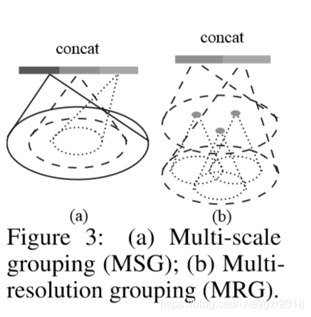
Multi-scale grouping (MSG):
多尺度特征学习,在Grouping layer使用不同的尺度,在PointNets 中捕获对应的尺度的特征,然后concat成一个多尺度特征。
在训练时候使用dropout,测试的时候,全部点都使用。
Multi-resolution grouping (MRG):(more efficient)
MSG的计算成本太高。MRG:still preserves the ability to adaptively aggregate information according to the distributional properties of points。
对于不同的level中的提取的特征做一个concat。
对照上图(b),新特征通过两部分连接起来。左边特征向量是通过一个set abstraction后得到的,右边特征向量是直接对当前patch(是指数据中的一小块)中所有点进行pointnet卷积得到。并且,当点云密度不均时,可以通过判断当前patch的密度对左右两个特征向量给予不同权重。例如,当patch中密度很小,左边向量得到的信息就没有对所有patch中点提取的特征可信度更高,于是将右特征向量的权重提高。以此达到减少计算量的同时解决密度问题。
五、分类网络结构
从图中可以看出,分类网络就是把lastest的set abstraction的特征输出作为全连接层的第一层数据,两层全连接之后实现40分类。下面代码使用的是SSG,即相同尺度特征,代码如下:
def get_model(point_cloud, is_training, bn_decay=None):
    """ Classification PointNet, input is BxNx3, output Bx40 """
    batch_size = point_cloud.get_shape()[0].value
    num_point = point_cloud.get_shape()[1].value
    end_points = {}
    l0_xyz = point_cloud # (16,1024,3)
    l0_points = None
    end_points['l0_xyz'] = l0_xyz

    # Set abstraction layers
    # Note: When using NCHW for layer 2, we see increased GPU memory usage (in TF1.4).
    # So we only use NCHW for layer 1 until this issue can be resolved.
    l1_xyz, l1_points, l1_indices = pointnet_sa_module(l0_xyz, l0_points, npoint=512, radius=0.2, nsample=32, mlp=[64,64,128], mlp2=None, group_all=False, is_training=is_training, bn_decay=bn_decay, scope='layer1', use_nchw=True)
    # l1_xyz = (16, 512, 3) 中心点
    # l1_points = (16, 512, 128) local region feature
    # l1_indices = (16, 512, 32) 512 center points(group), each group has 32 points
    l2_xyz, l2_points, l2_indices = pointnet_sa_module(l1_xyz, l1_points, npoint=128, radius=0.4, nsample=64, mlp=[128,128,256], mlp2=None, group_all=False, is_training=is_training, bn_decay=bn_decay, scope='layer2')
    # l2_xyz = (16, 128, 3)
    # l2_points = (16, 128, 256) local feature
    # l2_indices = (16, 128, 64)
    l3_xyz, l3_points, l3_indices = pointnet_sa_module(l2_xyz, l2_points, npoint=None, radius=None, nsample=None, mlp=[256,512,1024], mlp2=None, group_all=True, is_training=is_training, bn_decay=bn_decay, scope='layer3')
    # l3_xyz = (16, 1, 3)
    # l3_points = (16, 1, 1024) global feature
    # l3_indices = (16, 1, 128)
    # Fully connected layers
    # l3_points就是第三次sa的局部区域特征向量,d+C的那个
    net = tf.reshape(l3_points, [batch_size, -1])
    # 特征向量使用全连接1024-512
    net = tf_util.fully_connected(net, 512, bn=True, is_training=is_training, scope='fc1', bn_decay=bn_decay)
    net = tf_util.dropout(net, keep_prob=0.5, is_training=is_training, scope='dp1')
    #   512-256
    net = tf_util.fully_connected(net, 256, bn=True, is_training=is_training, scope='fc2', bn_decay=bn_decay)
    net = tf_util.dropout(net, keep_prob=0.5, is_training=is_training, scope='dp2')
    # 40分类
    net = tf_util.fully_connected(net, 40, activation_fn=None, scope='fc3')

    return net, end_points
六、分割网络结构
在set abstraction layer中,原始点是被子采样的。在分割任务中(如语义点标记),我们希望获得全部点的特征。
分割网络复杂一点,使用了skip link concatenation。
这部分先skip了。
七、说明
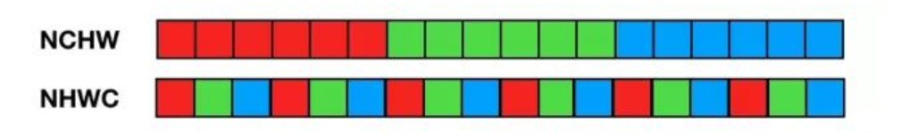
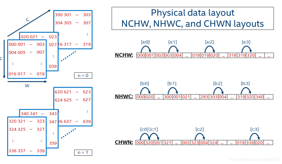
代码中提到数据的存储格式。
N代表数量, C代表channel,H代表高度,W代表宽度。NCHW其实代表的是[W H C N]。