算法：Rate of Growth

Rate of growth describes how an algorithm’s complexity changes as the input size grows. This is commonly represented using Big-O notation. Big-O notation uses a capital O (“order”) and a formula that expresses the complexity of the algorithm. The formula may have a variable, n, which represents the size of the input. The following are some common order functions we will see in this book but this list is by no means complete.

Constant – O(1)

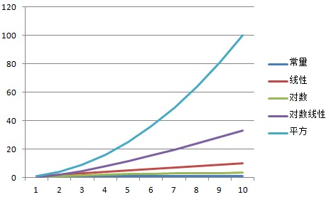
An O(1) algorithm is one whose complexity is constant regardless of how large the input size is. The 1 does not mean that there is only one operation or that the operation takes a small amount of time. It might take 1 microsecond or it might take 1 hour. The point is that the size of the input does not influence the time the operation takes.

        public int GetCount(int[] items)
        {
            return items.Length;
        }

Linear – O(n)

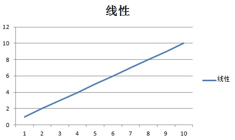
An O(n) algorithm is one whose complexity grows linearly with the size of the input. It is reasonable to expect that if an input size of 1 takes 5 milliseconds, an input with one thousand items will take 5 seconds.You can often recognize an O(n) algorithm by looking for a looping mechanism that accesses each member.

        public long GetSum(int[] items)
        {
            long sum = 0;
            foreach (int i in items)
            {
                sum += i;
            } 
            return sum;
        }

Logarithmic – O(log n)

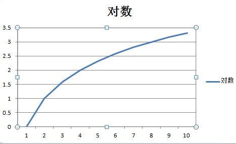
 An O(log n) algorithm is one whose complexity is logarithmic to its size. Many divide and conquer algorithms fall into this bucket. The binary search tree Contains method implements an O(log n) algorithm.

Linearithmic – O(n log n)

A linearithmic algorithm, or loglinear, is an algorithm that has a complexity of O(n log n). Some divide and conquer algorithms fall into this bucket. We will see two examples when we look at merge sort and quick sort.

An O(n2)

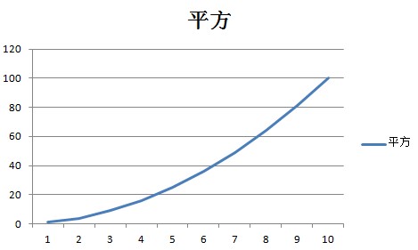
An O(n2) algorithm is one whose complexity is quadratic to its size. While not always avoidable, using a quadratic algorithm is a potential sign that you need to reconsider your algorithm or data structure choice. Quadratic algorithms do not scale well as the input size grows. For example, an array with 1000 integers would require 1,000,000 operations to complete. An input with one million items would take one trillion (1,000,000,000,000) operations. To put this into perspective, if each operation takes one millisecond to complete, an O(n2) algorithm that receives an input of one million items will take nearly 32 years to complete. Making that algorithm 100 times faster would still take 84 days.
We will see an example of a quadratic algorithm when we look at bubble sort.

Best, Average, and Worst Case

When we say an algorithm is O(n), what are we really saying? Are we saying that the algorithm is O(n) on average? Or are we describing the best or worst case scenario?

We typically mean the worst case scenario unless the common case and worst case are vastly different. For example, we will see examples in this book where an algorithm is O(1) on average, but periodically becomes O(n) (see ArrayList.Add). In these cases I will describe the algorithm as O(1) on average and then explain when the complexity changes.

The key point is that saying O(n) does not mean that it is always n operations. It might be less, but it should not be more.

What are we Measuring?

When we are measuring algorithms and data structures, we are usually talking about one of two things: the amount of time the operation takes to complete (operational complexity), or the amount of resources (memory) an algorithm uses (resource complexity).

An algorithm that runs ten times faster but uses ten times as much memory might be perfectly acceptable in a server environment with vast amounts of available memory, but may not be appropriate in an embedded environment where available memory is severely limited.

In this book I will focus primarily on operational complexity, but in the Sorting Algorithms chapter we will see some examples of resource complexity.

Some specific examples of things we might measure include:

• Comparison operations (greater than, less than, equal to).
• Assignments and data swapping.
• Memory allocations.

The context of the operation being performed will typically tell you what type of measurement is being made.

For example, when discussing the complexity of an algorithm that searches for an item within a data structure, we are almost certainly talking about comparison operations. Search is generally a read-only operation so there should not be any need to perform assignments or allocate memory.

However, when we are talking about data sorting it might be logical to assume that we could be talking about comparisons, assignments, or allocations. In cases where there may be ambiguity, I will indicate which type of measurement the complexity is actually referring to.