Matlab vs Python 作图

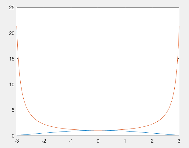
-- Matlab 作图示例

x=-3:0.00003:3;

y1=sin(x)./x;

y2=x./sin(x);

plot(x,y1,x,y2);

-- Python 作图示例

import numpy as np
import matplotlib.pyplot as plt

x = np.arange(-3, 3, 0.00003)
y1 = 1/(np.sin(x)) * x
y2 = (np.sin(x)) / x

plt.plot(x, y1, x, y2)
plt.show()

 

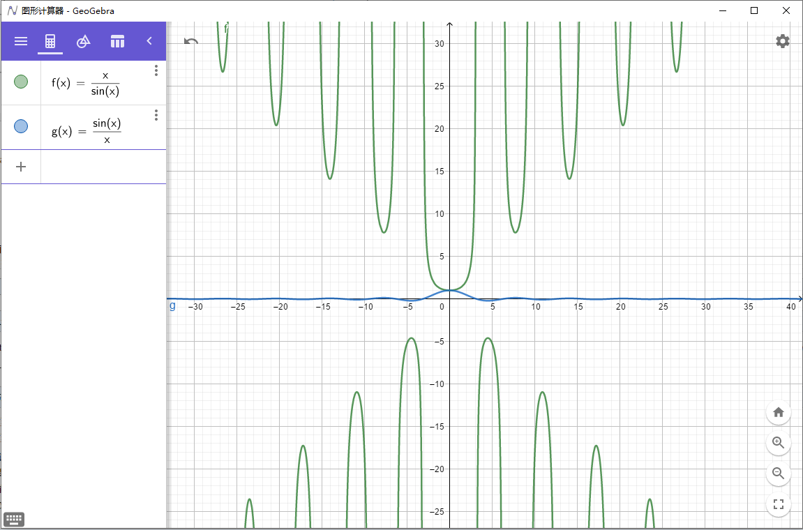
GeoGebra 工具作图：

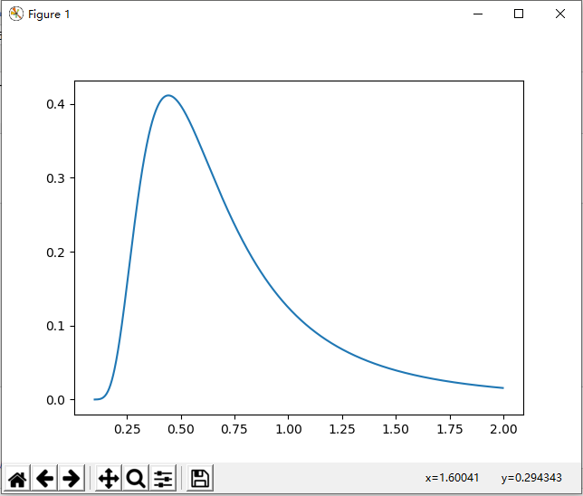
python 画普朗克线（黑体辐射）：

import numpy as np
import matplotlib.pyplot as plt

x = np.arange(0.1, 2, 0.002)
y1=1/x**5/(np.exp(2.2/x)-1)

plt.plot(x, y1)
plt.show()

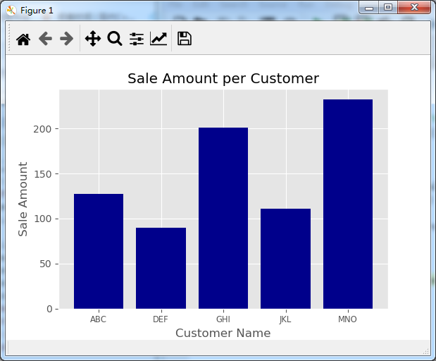
书本示例：

1、条形图

#!/usr/bin/env_python3
import matplotlib.pyplot as plt
plt.style.use('ggplot')
customers = ['ABC','DEF','GHI','JKL','MNO']
#生成序列：0,1,2,3,4
customers_index = range(len(customers))
sale_amounts = [127,90,201,111,232]
fig=plt.figure()
ax1=fig.add_subplot(1,1,1)
ax1.bar(customers_index,sale_amounts,align='center',color='darkblue')
ax1.xaxis.set_ticks_position('bottom')
ax1.yaxis.set_ticks_position('left')
#设置x轴显示值为customers
plt.xticks(customers_index,customers,rotation=0,fontsize='small')
plt.xlabel('Customer Name')
plt.ylabel('Sale Amount')
plt.title('Sale Amount per Customer')
#保存图片
plt.savefig('bar_plot.png',dpi=400,bbox_inches='tight')
plt.show()

 2、直方图

import numpy as np
import matplotlib.pyplot as plt

plt.style.use('ggplot')

#随机种子，一旦随机种子参数确定，np.random.randn生成的结果也确定
np.random.seed(19680801)

#生成正态分布数据
mu=100 #正态分布均值点
sigma=15 #正态分布标准差
x=mu1+sigma*np.random.randn(10000) #np.random.randn标准正态分布随机值

num_bins=50 #histogram组数，即柱子的个数

fig,ax=plt.subplots()

#the histogram of the data
#n 表示每个bin的值
#bins,shape为n+1,bins的边界
#patcher histogram中每一个柱子
#生成的直方图面积和为1,即sum(n*(bins[1:]-bins[-1]))==1
n,bins,patches=ax.hist(x,num_bins,density=1,color='darkgreen')

#正态分布拟合曲线
y=((1/(np.sqrt(2*np.pi)*sigma))*np.exp(-0.5*(1/sigma*(bins-mu))**2))
ax.plot(bins,y,'--') #画直线

plt.xlabel('Abscissa labels') #横坐标label
plt.ylabel('Probability density') #纵坐标label
ax.set_title(r'Histogram of IQ: $mu=100$, $sigma=15$')  #设置标题
ax.xaxis.set_ticks_position('bottom') #设置坐标轴显示位置
ax.yaxis.set_ticks_position('left')
fig.set_facecolor('cyan')  #设置figure面板颜色(青色)

#plt.savefig('historgram.png',dpi=400,bbox_inches='tight')
plt.show()

  

matplotlib 官方文档：https://matplotlib.org/mpl_toolkits/mplot3d/tutorial.html

参考书本：《Python 数据分析基础》陈光欣 译