课程一(Neural Networks and Deep Learning)，第二周（Basics of Neural Network programming）—— 3、Python Basics with numpy (optional)

Python Basics with numpy (optional)
Welcome to your first (Optional) programming exercise of the deep learning specialization. In this assignment you will:

- Learn how to use numpy.

- Implement some basic core deep learning functions such as the softmax, sigmoid, dsigmoid, etc...

- Learn how to handle data by normalizing inputs and reshaping images.

- Recognize the importance of vectorization.

- Understand how python broadcasting works.

This assignment prepares you well for the upcoming assignment. Take your time to complete it and make sure you get the expected outputs when working through the different exercises. In some code blocks, you will find a "#GRADED FUNCTION: functionName" comment. Please do not modify it. After you are done, submit your work and check your results. You need to score 70% to pass. Good luck :) !

中文翻译------------>

numpy 的 Python 基础知识 (可选)

欢迎您的第一次 (可选) 编程练习的深度学习专门化。在本作业中, 您将:

-学习如何使用 numpy。

-实施一些基本的核心学习功能, 如 softmax、 sigmoid、dsigmoid 等。

-了解如何通过规范化输入和重塑图像来处理数据。

-认识到向量化的重要性。

-了解 python 广播的工作原理。

这个任务为即将到来的任务做好准备。用你的时间完成它, 通过不同的练习，确保你得到预期的结果, 。在某些代码块中, 您将找到一个 ""#GRADED FUNCTION: functionName" 的注释。请不要修改它。完成后, 提交您的工作, 并检查您的结果。你需要得分70% 才能过关。祝你好运:)!

--------------------------------------------------------------------------------------------------------------------------------------

Welcome to your first assignment. This exercise gives you a brief introduction to Python. Even if you've used Python before, this will help familiarize you with functions we'll need.
Instructions:
You will be using Python 3.
Avoid using for-loops and while-loops, unless you are explicitly told to do so.
Do not modify the (# GRADED FUNCTION [function name]) comment in some cells. Your work would not be graded if you change this. Each cell containing that comment should only contain one function.
After coding your function, run the cell right below it to check if your result is correct.
After this assignment you will:
Be able to use iPython Notebooks
Be able to use numpy functions and numpy matrix/vector operations
Understand the concept of "broadcasting"
Be able to vectorize code
Let's get started!

中文翻译------------>

欢迎您的第一次任务。本练习将简要介绍 Python。即使您以前使用过 Python, 这将有助于您熟悉我们需要的功能。

说明:

您将使用 Python 3。

避免使用 for 循环和循环, 除非明确告诉你这样做。

不要修改某些单元格中的 (# GRADED FUNCTION [function name]) 注释。如果你改变了这一点, 你的工作将不会被评分。包含该注释的每个单元格只应包含一个函数。

在对函数进行编码后, 运行下面的单元格, 检查结果是否正确。

完成此任务后, 您将:

能够使用 iPython 笔记本

能够使用 numpy 函数和 numpy 矩阵/向量运算

理解 "广播" 的概念

能够向量化代码

我们开始吧!

--------------------------------------------------------------------------------------------------------------------------------------

About iPython Notebooks
iPython Notebooks are interactive coding environments embedded in a webpage. You will be using iPython notebooks in this class. You only need to write code between the ### START CODE HERE ### and ### END CODE HERE ### comments. After writing your code, you can run the cell by either pressing "SHIFT"+"ENTER" or by clicking on "Run Cell" (denoted by a play symbol) in the upper bar of the notebook.
We will often specify "(≈ X lines of code)" in the comments to tell you about how much code you need to write. It is just a rough estimate, so don't feel bad if your code is longer or shorter.

中文翻译------------>

关于 iPython 笔记本

iPython 笔记本是嵌入在网页中的交互式编码环境。您将在本课中使用 iPython 笔记本。您只需要在 ### START CODE HERE ### and ### END CODE HERE ### 编写代码, 然后可以通过按 "SHIFT" + "ENTER" 或在笔记本的上部栏中单击 "Run Cell"  (由播放符号表示) 来运行单元格。

我们经常会在注释中指定 "(≈ X 行代码)" 来告诉您需要编写多少代码。这只是一个粗略的估计, 所以如果您的代码更长或更短, 请不要感到遗憾。

 

--------------------------------------------------------------------------------------------------------------------------------------

Exercise: Set test to "Hello World" in the cell below to print "Hello World" and run the two cells below.

中文翻译------------>

练习: 将测试设置为 "Hello World", 在下面的单元格中打印 "Hello World"并运行下面的两个单元格。

code--------->

### START CODE HERE ### (≈ 1 line of code)
test = "Hello World"
### END CODE HERE ###

print ("test: " + test)

Expected output: test: Hello World

 

--------------------------------------------------------------------------------------------------------------------------------------

What you need to remember:
Run your cells using SHIFT+ENTER (or "Run cell")
Write code in the designated areas using Python 3 only
Do not modify the code outside of the designated areas

中文翻译------------>

您需要记住的内容:

使用 SHIFT + ENTER(或 "Run cell") 运行单元格

仅使用 Python 3 在指定区域中编写代码

不要修改指定区域之外的代码

--------------------------------------------------------------------------------------------------------------------------------------

1 - Building basic functions with numpy

Numpy is the main package for scientific computing in Python. It is maintained by a large community (www.numpy.org). In this exercise you will learn several key numpy functions such as np.exp, np.log, and np.reshape. You will need to know how to use these functions for future assignments.

1.1 - sigmoid function, np.exp()

Before using np.exp(), you will use math.exp() to implement the sigmoid function. You will then see why np.exp() is preferable to math.exp().

Exercise: Build a function that returns the sigmoid of a real number x. Use math.exp(x) for the exponential function.
Reminder: sigmoid(x)=is sometimes also known as the logistic function. It is a non-linear function used not only in Machine Learning (Logistic Regression), but also in Deep Learning.

To refer to a function belonging to a specific package you could call it using package_name.function(). Run the code below to see an example with math.exp().

中文翻译------------>

1-建设基本功能与 numpy

Numpy 是 Python 中科学计算的主要软件包。它由一个大社区维护 (www.numpy.org)。在本练习中, 您将学习一些关键的 numpy 函数, 如 np. exp、np.log 和 np.reshape。您需要知道如何将这些函数用于将来的作业。

1.1-sigmoid function, np.exp()

在使用 np. exp () 之前, 您将使用math. exp () 来实现sigmoid 函数。然后你就会明白为什么 np.exp() 比math.exp()更好了。

 

练习: 生成返回实数 x 的sigmoid函数. 使用 math.exp(x)来代替指数。

提示: sigmoid(x)=有时也称为逻辑函数。它是一种非线性函数, 不仅用于机器学习 (逻辑回归), 而且还用于深度学习。

要引用属于特定包的函数, 可以使用 package_name.function()来调用它。运行下面的代码以查看math. exp () 的示例。

 

code--------->

# GRADED FUNCTION: basic_sigmoid

import math

def basic_sigmoid(x):
    """
    Compute sigmoid of x.

    Arguments:
    x -- A scalar

    Return:
    s -- sigmoid(x)
    """
    
    ### START CODE HERE ### (≈ 1 line of code)
    s = 1/(1+math.exp(-x))
    ### END CODE HERE ###
    
    return s

basic_sigmoid(3)

Expected Output:

basic_sigmoid(3)

0.9525741268224334

--------------------------------------------------------------------------------------------------------------------------------------

 Actually, we rarely use the "math" library in deep learning because the inputs of the functions are real numbers. In deep learning we mostly use matrices and vectors. This is why numpy is more useful.

 

中文翻译------------>

实际上, 我们很少在深入学习中使用 "math" 库, 因为函数的输入是实数。在深入学习中, 我们主要使用矩阵和向量。这就是为什么 numpy 更有用。

 

 code--------->

### One reason why we use "numpy" instead of "math" in Deep Learning ###
x = [1, 2, 3]
basic_sigmoid(x) 
# you will see this give an error when you run it, because x is a vector.

---------------------------------------------------------------------------
TypeError                                 Traceback (most recent call last)
<ipython-input-6-2e11097d6860> in <module>()
      1 ### One reason why we use "numpy" instead of "math" in Deep Learning ###
      2 x = [1, 2, 3]
----> 3 basic_sigmoid(x) # you will see this give an error when you run it, because x is a vector.

<ipython-input-4-951c5721dbfa> in basic_sigmoid(x)
     15 
     16     ### START CODE HERE ### (≈ 1 line of code)
---> 17     s = 1/(1+math.exp(-x))
     18     ### END CODE HERE ###
     19 

TypeError: bad operand type for unary -: 'list'

 In fact, if x=(x₁,x₂,...,x_n) is a row vector then np.exp(x)will apply the exponential function to every element of x. The output will thus be: np.exp(x)=(e^x1,e^x2,...,e^xn)

 

import numpy as np

# example of np.exp
x = np.array([1, 2, 3])
print(np.exp(x)) # result is (exp(1), exp(2), exp(3))

 result:

[  2.71828183   7.3890561   20.08553692]

 Furthermore, if x is a vector, then a Python operation such as s=x+3s=x+3 or s=1xs=1x will output s as a vector of the same size as x.

# example of vector operation
x = np.array([1, 2, 3])
print (x + 3)

  result:

[4 5 6]

--------------------------------------------------------------------------------------------------------------------------------------

Any time you need more info on a numpy function, we encourage you to look at the official documentation.
You can also create a new cell in the notebook and write np.exp? (for example) to get quick access to the documentation.

中文翻译------------>

任何时候, 你需要更多的信息 numpy 功能, 我们鼓励你看看官方文件。

您还可以在笔记本中创建一个新单元, 并编写 np. exp？(例如) 获取文档的快速访问。

--------------------------------------------------------------------------------------------------------------------------------------

 

Exercise: Implement the sigmoid function using numpy.
Instructions: x could now be either a real number, a vector, or a matrix. The data structures we use in numpy to represent these shapes (vectors, matrices...) are called numpy arrays. You don't need to know more for now.

中文翻译------------>

练习: 使用 numpy 实现sigmoid函数。

说明: x 现在可以是实数、向量或矩阵。我们在 numpy 中使用的数据结构来表示这些形状 (向量、矩阵......) 称为 numpy 数组。你现在不需要知道更多。

code----------->

# GRADED FUNCTION: sigmoid

import numpy as np # this means you can access numpy functions by writing np.function() instead of numpy.function()

def sigmoid(x):
    """
    Compute the sigmoid of x

    Arguments:
    x -- A scalar or numpy array of any size

    Return:
    s -- sigmoid(x)
    """
    
    ### START CODE HERE ### (≈ 1 line of code)
    s = 1/(1+np.exp(-x))
    ### END CODE HERE ###
    
    return s

x = np.array([1, 2, 3])

# x=[1,2,3]   #这种写法会报错

sigmoid(x)

result:

array([ 0.73105858,  0.88079708,  0.95257413])

Expected Output:

sigmoid([1,2,3])

array([ 0.73105858, 0.88079708, 0.95257413])

--------------------------------------------------------------------------------------------------------------------------------------

1.2 - Sigmoid gradient

As you've seen in lecture, you will need to compute gradients to optimize loss functions using backpropagation. Let's code your first gradient function.

中文翻译------------>

1.2-Sigmoid 的导数

正如您在讲座中所看到的, 您将需要使用反向传播计算导数以优化损失函数。让我们为您的第一个导数编写代码。

 

Exercise: Implement the function sigmoid_grad() to compute the gradient of the sigmoid function with respect to its input x. The formula is:

　　sigmoid_derivative(x)=σ′(x)=σ(x)(1−σ(x))                                (2)

You often code this function in two steps:

1. Set s to be the sigmoid of x. You might find your sigmoid(x) function useful.
2. Compute σ′(x)=s(1−s)σ′(x)=s(1−s)

# GRADED FUNCTION: sigmoid_derivative

def sigmoid_derivative(x):
    """
    Compute the gradient (also called the slope or derivative) of the sigmoid function with respect to its input x.
    You can store the output of the sigmoid function into variables and then use it to calculate the gradient.
    
    Arguments:
    x -- A scalar or numpy array

    Return:
    ds -- Your computed gradient.
    """
    
    ### START CODE HERE ### (≈ 2 lines of code)
    s = 1/(1+np.exp(-x))
    ds = s*(1-s)
    ### END CODE HERE ###
    
    return ds

   x = np.array([1, 2, 3])
    print ("sigmoid_derivative(x) = " + str(sigmoid_derivative(x)))

result:

sigmoid_derivative(x) = [ 0.19661193  0.10499359  0.04517666]

Expected Output:

sigmoid_derivative([1,2,3])

[ 0.19661193 0.10499359 0.04517666]

--------------------------------------------------------------------------------------------------------------------------------------

1.3 - Reshaping arrays

Two common numpy functions used in deep learning are np.shape and np.reshape().

• X.shape is used to get the shape (dimension) of a matrix/vector X.
• X.reshape(...) is used to reshape X into some other dimension.

For example, in computer science, an image is represented by a 3D array of shape (length,height,depth=3). However, when you read an image as the input of an algorithm you convert it to a vector of shape (length∗height∗3,1). In other words, you "unroll", or reshape, the 3D array into a 1D vector.

中文翻译------------>

1.3-修改数组的形状 

在深度学习中, 常用的两种 numpy 函数是 np.shape 和 np.reshape().

　　x. shape用于获取矩阵的形状 (尺寸)

　　x.reshape(...) 用于将 X 重塑为其他维度。

例如, 在计算机科学中, 一个图像由一个3D 的形状数组 (length,height,depth=3) 表示。但是, 当您将图像作为算法的输入进行读取时, 将其转换为一维的列向量 (length∗height∗3,1)。换言之, 您将3D 数组 "展开" 或重塑为1D 向量。

Exercise: Implement image2vector() that takes an input of shape (length, height, 3) and returns a vector of shape (length*height*3, 1). For example, if you would like to reshape an array v of shape (a, b, c) into a vector of shape (a*b,c) you would do:

v = v.reshape((v.shape[0]*v.shape[1], v.shape[2])) # v.shape[0] = a ; v.shape[1] = b ; v.shape[2] = c

• Please don't hardcode the dimensions of image as a constant. Instead look up the quantities you need with image.shape[0], etc.

中文翻译------------>

练习: 实现 image2vector (), 它接受维度为(长度、高度、3)的输入， 并返回维度为 (length*height*3, 1)的向量。例如, 如果您想将维度 (a，b，c) 的数组 v 转换为向量 (a * b, c), 您将执行以下操作:

v = v.reshape((v.shape[0]*v.shape[1], v.shape[2])) # v.shape[0] = a ; v.shape[1] = b ; v.shape[2] = c

请不要将图像的尺寸定为常量。而是用image.shape[0]等查找所需的数量。

 

code--------------->

# GRADED FUNCTION: image2vector
def image2vector(image):
    """
    Argument:
    image -- a numpy array of shape (length, height, depth)
    
    Returns:
    v -- a vector of shape (length*height*depth, 1)
    """
    
    ### START CODE HERE ### (≈ 1 line of code)
    v = image.reshape(image.shape[0]*image.shape[1]*image.shape[2],1)
    ### END CODE HERE ###
    
    return v

# This is a 3 by 3 by 2 array, typically images will be (num_px_x, num_px_y,3) where 3 represents the RGB values
image = np.array([[[ 0.67826139,  0.29380381],
        [ 0.90714982,  0.52835647],
        [ 0.4215251 ,  0.45017551]],

       [[ 0.92814219,  0.96677647],
        [ 0.85304703,  0.52351845],
        [ 0.19981397,  0.27417313]],

       [[ 0.60659855,  0.00533165],
        [ 0.10820313,  0.49978937],
        [ 0.34144279,  0.94630077]]])

print ("image2vector(image) = " + str(image2vector(image)))

result:

image2vector(image) = [[ 0.67826139]
 [ 0.29380381]
 [ 0.90714982]
 [ 0.52835647]
 [ 0.4215251 ]
 [ 0.45017551]
 [ 0.92814219]
 [ 0.96677647]
 [ 0.85304703]
 [ 0.52351845]
 [ 0.19981397]
 [ 0.27417313]
 [ 0.60659855]
 [ 0.00533165]
 [ 0.10820313]
 [ 0.49978937]
 [ 0.34144279]
 [ 0.94630077]]

Expected Output:

image2vector(image)

[[ 0.67826139] [ 0.29380381] [ 0.90714982] [ 0.52835647] [ 0.4215251 ] [ 0.45017551] [ 0.92814219] [ 0.96677647] [ 0.85304703] [ 0.52351845] [ 0.19981397] [ 0.27417313] [ 0.60659855] [ 0.00533165] [ 0.10820313] [ 0.49978937] [ 0.34144279] [ 0.94630077]]

-------------------------------------------------------------------------------------------------------------------------------------------------------------

1.4 - Normalizing rows

Another common technique we use in Machine Learning and Deep Learning is to normalize our data. It often leads to a better performance because gradient descent converges faster after normalization. Here, by normalization we mean changing x to(dividing each row vector of x by its norm).

For example, if

then

and

Note that you can divide matrices of different sizes and it works fine: this is called broadcasting and you're going to learn about it in part 5.

 中文翻译------------>

1.4 - 标准化行向量

我们在机器学习和深入学习中使用的另一项常用技术是规范我们的数据。它通常会导致更好的性能, 因为渐变下降在正常化后收敛得更快。在这里, 通过规范化, 我们的意思是改变 x 到  (除以行向量的2-范数除以每行向量)。

例如, 如果

那么

并且

请注意, 您可以除以不同大小的矩阵, 而且会正常运行: 这叫做广播, 您将在part5中了解它。

 

Exercise: Implement normalizeRows() to normalize the rows of a matrix. After applying this function to an input matrix x, each row of x should be a vector of unit length (meaning length 1).

 中文翻译------------>

练习: 实现 normalizeRows () 来规范化矩阵的行。在将此函数应用于输入矩阵 x 之后, x 的每一行都应该是单位长度的向量 (意思是长度 1)。

code----------------->

# GRADED FUNCTION: normalizeRows

def normalizeRows(x):
    """
    Implement a function that normalizes each row of the matrix x (to have unit length).
    
    Argument:
    x -- A numpy matrix of shape (n, m)
    
    Returns:
    x -- The normalized (by row) numpy matrix. You are allowed to modify x.
    """
    
    ### START CODE HERE ### (≈ 2 lines of code)
    # Compute x_norm as the norm 2 of x. Use np.linalg.norm(..., ord = 2, axis = ..., keepdims = True)
    x_norm = np.linalg.norm(x,axis=1,keepdims=True)
    
    # Divide x by its norm.
    x = x/x_norm
    ### END CODE HERE ###

    return x

x = np.array([
    [0, 3, 4],
    [1, 6, 4]])
print("normalizeRows(x) = " + str(normalizeRows(x)))

result:

normalizeRows(x) = [[ 0.          0.6         0.8       ]
 [ 0.13736056  0.82416338  0.54944226]]

Expected Output:

normalizeRows(x)

[[ 0. 0.6 0.8 ] [ 0.13736056 0.82416338 0.54944226]]

Note: In normalizeRows(), you can try to print the shapes of x_norm and x, and then rerun the assessment. You'll find out that they have different shapes. This is normal given that x_norm takes the norm of each row of x. So x_norm has the same number of rows but only 1 column. So how did it work when you divided x by x_norm? This is called broadcasting and we'll talk about it now!

-------------------------------------------------------------------------------------------------------------------------------------------------------------

1.5 - Broadcasting and the softmax function

A very important concept to understand in numpy is "broadcasting". It is very useful for performing mathematical operations between arrays of different shapes. For the full details on broadcasting, you can read the official broadcasting documentation.

Exercise: Implement a softmax function using numpy. You can think of softmax as a normalizing function used when your algorithm needs to classify two or more classes. You will learn more about softmax in the second course of this specialization.

Instructions:

 中文翻译------------>

一个非常重要的概念是要理解numpy中的"广播"。它对于在不同形状的数组之间执行数学运算非常有用。关于广播的全部细节, 你可以阅读官方的广播文档。

练习: 使用 numpy 实现 softmax 函数。当您的算法需要对两个或多个类进行分类时, 可以将 softmax 视为正则函数。在这一专业的第二门课中, 您将了解更多关于 softmax 的信息。

code----------------->

# GRADED FUNCTION: softmax

def softmax(x):
    """Calculates the softmax for each row of the input x.

    Your code should work for a row vector and also for matrices of shape (n, m).

    Argument:
    x -- A numpy matrix of shape (n,m)

    Returns:
    s -- A numpy matrix equal to the softmax of x, of shape (n,m)
    """
    
    ### START CODE HERE ### (≈ 3 lines of code)
    # Apply exp() element-wise to x. Use np.exp(...).
    x_exp = np.exp(x)

    # Create a vector x_sum that sums each row of x_exp. Use np.sum(..., axis = 1, keepdims = True).
    x_sum = np.sum(x_exp,axis=1,keepdims=True)
    
    # Compute softmax(x) by dividing x_exp by x_sum. It should automatically use numpy broadcasting.
    s = x_exp/x_sum

    ### END CODE HERE ###
    
    return s

x = np.array([
    [9, 2, 5, 0, 0],
    [7, 5, 0, 0 ,0]])
print("softmax(x) = " + str(softmax(x)))

result:

softmax(x) = [[  9.80897665e-01   8.94462891e-04   1.79657674e-02   1.21052389e-04
    1.21052389e-04]
 [  8.78679856e-01   1.18916387e-01   8.01252314e-04   8.01252314e-04
    8.01252314e-04]]

Expected Output:

softmax(x)

[[ 9.80897665e-01 8.94462891e-04 1.79657674e-02 1.21052389e-04 1.21052389e-04] [ 8.78679856e-01 1.18916387e-01 8.01252314e-04 8.01252314e-04 8.01252314e-04]]

 

Note:

• If you print the shapes of x_exp, x_sum and s above and rerun the assessment cell, you will see that x_sum is of shape (2,1) while x_exp and s are of shape (2,5). x_exp/x_sum works due to python broadcasting.

Congratulations! You now have a pretty good understanding of python numpy and have implemented a few useful functions that you will be using in deep learning.

What you need to remember:

• np.exp(x) works for any np.array x and applies the exponential function to every coordinate
• the sigmoid function and its gradient
• image2vector is commonly used in deep learning
• np.reshape is widely used. In the future, you'll see that keeping your matrix/vector dimensions straight will go toward eliminating a lot of bugs.
• numpy has efficient built-in functions
• broadcasting is extremely useful

-----------------------------------------------------------------------------------------------------------------------------------------------------

2) Vectorization

In deep learning, you deal with very large datasets. Hence, a non-computationally-optimal function can become a huge bottleneck in your algorithm and can result in a model that takes ages to run. To make sure that your code is computationally efficient, you will use vectorization. For example, try to tell the difference between the following implementations of the dot/outer/elementwise product.

中文翻译------->

2) 矢量化

 在深度学习中, 您将处理非常大的数据集。因此, 没有经过优化的函数可能会成为算法中的一个巨大瓶颈, 并可能导致一个模型需要运行很长时间。为了确保您的代码在计算上有效, 您将使用向量化。例如, 尝试区分以下运算的区别。

code---------->

import time

x1 = [9, 2, 5, 0, 0, 7, 5, 0, 0, 0, 9, 2, 5, 0, 0]
x2 = [9, 2, 2, 9, 0, 9, 2, 5, 0, 0, 9, 2, 5, 0, 0]

### CLASSIC DOT PRODUCT OF VECTORS IMPLEMENTATION ###
tic = time.process_time()
dot = 0
for i in range(len(x1)):
    dot+= x1[i]*x2[i]
toc = time.process_time()
print ("dot = " + str(dot) + "
 ----- Computation time = " + str(1000*(toc - tic)) + "ms")

### CLASSIC OUTER PRODUCT IMPLEMENTATION ###
tic = time.process_time()
outer = np.zeros((len(x1),len(x2))) # we create a len(x1)*len(x2) matrix with only zeros
for i in range(len(x1)):
    for j in range(len(x2)):
        outer[i,j] = x1[i]*x2[j]
toc = time.process_time()
print ("outer = " + str(outer) + "
 ----- Computation time = " + str(1000*(toc - tic)) + "ms")

### CLASSIC ELEMENTWISE IMPLEMENTATION ###
tic = time.process_time()
mul = np.zeros(len(x1))
for i in range(len(x1)):
    mul[i] = x1[i]*x2[i]
toc = time.process_time()
print ("elementwise multiplication = " + str(mul) + "
 ----- Computation time = " + str(1000*(toc - tic)) + "ms")

### CLASSIC GENERAL DOT PRODUCT IMPLEMENTATION ###
W = np.random.rand(3,len(x1)) # Random 3*len(x1) numpy array
tic = time.process_time()
gdot = np.zeros(W.shape[0])  #W.shape[0]=3
for i in range(W.shape[0]):  #W的每一行与x1进行点乘
    for j in range(len(x1)):
        gdot[i] += W[i,j]*x1[j]
toc = time.process_time()
print ("gdot = " + str(gdot) + "
 ----- Computation time = " + str(1000*(toc - tic)) + "ms")

result:

dot = 278
 ----- Computation time = 0.180011000000313ms
outer = [[ 81.  18.  18.  81.   0.  81.  18.  45.   0.   0.  81.  18.  45.   0.
    0.]
 [ 18.   4.   4.  18.   0.  18.   4.  10.   0.   0.  18.   4.  10.   0.
    0.]
 [ 45.  10.  10.  45.   0.  45.  10.  25.   0.   0.  45.  10.  25.   0.
    0.]
 [  0.   0.   0.   0.   0.   0.   0.   0.   0.   0.   0.   0.   0.   0.
    0.]
 [  0.   0.   0.   0.   0.   0.   0.   0.   0.   0.   0.   0.   0.   0.
    0.]
 [ 63.  14.  14.  63.   0.  63.  14.  35.   0.   0.  63.  14.  35.   0.
    0.]
 [ 45.  10.  10.  45.   0.  45.  10.  25.   0.   0.  45.  10.  25.   0.
    0.]
 [  0.   0.   0.   0.   0.   0.   0.   0.   0.   0.   0.   0.   0.   0.
    0.]
 [  0.   0.   0.   0.   0.   0.   0.   0.   0.   0.   0.   0.   0.   0.
    0.]
 [  0.   0.   0.   0.   0.   0.   0.   0.   0.   0.   0.   0.   0.   0.
    0.]
 [ 81.  18.  18.  81.   0.  81.  18.  45.   0.   0.  81.  18.  45.   0.
    0.]
 [ 18.   4.   4.  18.   0.  18.   4.  10.   0.   0.  18.   4.  10.   0.
    0.]
 [ 45.  10.  10.  45.   0.  45.  10.  25.   0.   0.  45.  10.  25.   0.
    0.]
 [  0.   0.   0.   0.   0.   0.   0.   0.   0.   0.   0.   0.   0.   0.
    0.]
 [  0.   0.   0.   0.   0.   0.   0.   0.   0.   0.   0.   0.   0.   0.
    0.]]
 ----- Computation time = 0.33128299999996ms
elementwise multiplication = [ 81.   4.  10.   0.   0.  63.  10.   0.   0.   0.  81.   4.  25.   0.   0.]
 ----- Computation time = 0.1852840000000633ms
gdot = [ 16.77194969  27.17079675   9.70245758]
 ----- Computation time = 0.2552120000001157ms

x1 = [9, 2, 5, 0, 0, 7, 5, 0, 0, 0, 9, 2, 5, 0, 0]
x2 = [9, 2, 2, 9, 0, 9, 2, 5, 0, 0, 9, 2, 5, 0, 0]

### VECTORIZED DOT PRODUCT OF VECTORS ###
tic = time.process_time()
dot = np.dot(x1,x2)
toc = time.process_time()
print ("dot = " + str(dot) + "
 ----- Computation time = " + str(1000*(toc - tic)) + "ms")

### VECTORIZED OUTER PRODUCT ###
tic = time.process_time()
outer = np.outer(x1,x2)
toc = time.process_time()
print ("outer = " + str(outer) + "
 ----- Computation time = " + str(1000*(toc - tic)) + "ms")

### VECTORIZED ELEMENTWISE MULTIPLICATION ###
tic = time.process_time()
mul = np.multiply(x1,x2)
toc = time.process_time()
print ("elementwise multiplication = " + str(mul) + "
 ----- Computation time = " + str(1000*(toc - tic)) + "ms")

### VECTORIZED GENERAL DOT PRODUCT ###
tic = time.process_time()
dot = np.dot(W,x1)   # W的每一行与x1进行点乘
toc = time.process_time()
print ("gdot = " + str(dot) + "
 ----- Computation time = " + str(1000*(toc - tic)) + "ms")

result:

dot = 278
 ----- Computation time = 0.17461499999971153ms
outer = [[81 18 18 81  0 81 18 45  0  0 81 18 45  0  0]
 [18  4  4 18  0 18  4 10  0  0 18  4 10  0  0]
 [45 10 10 45  0 45 10 25  0  0 45 10 25  0  0]
 [ 0  0  0  0  0  0  0  0  0  0  0  0  0  0  0]
 [ 0  0  0  0  0  0  0  0  0  0  0  0  0  0  0]
 [63 14 14 63  0 63 14 35  0  0 63 14 35  0  0]
 [45 10 10 45  0 45 10 25  0  0 45 10 25  0  0]
 [ 0  0  0  0  0  0  0  0  0  0  0  0  0  0  0]
 [ 0  0  0  0  0  0  0  0  0  0  0  0  0  0  0]
 [ 0  0  0  0  0  0  0  0  0  0  0  0  0  0  0]
 [81 18 18 81  0 81 18 45  0  0 81 18 45  0  0]
 [18  4  4 18  0 18  4 10  0  0 18  4 10  0  0]
 [45 10 10 45  0 45 10 25  0  0 45 10 25  0  0]
 [ 0  0  0  0  0  0  0  0  0  0  0  0  0  0  0]
 [ 0  0  0  0  0  0  0  0  0  0  0  0  0  0  0]]
 ----- Computation time = 0.14286900000004543ms
elementwise multiplication = [81  4 10  0  0 63 10  0  0  0 81  4 25  0  0]
 ----- Computation time = 0.11042900000002298ms
gdot = [ 16.77194969  27.17079675   9.70245758]
 ----- Computation time = 0.17551299999984948ms

As you may have noticed, the vectorized implementation is much cleaner and more efficient. For bigger vectors/matrices, the differences in running time become even bigger.

Note that np.dot() performs a matrix-matrix or matrix-vector multiplication. This is different from np.multiply() and the * operator (which is equivalent to .* in Matlab/Octave), which performs an element-wise multiplication.

------------------------------------------------------------------------------------------------------------------------------

2.1 Implement the L1 and L2 loss functions

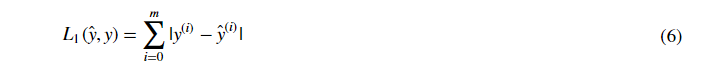
Exercise: Implement the numpy vectorized version of the L1 loss. You may find the function abs(x) (absolute value of x) useful.

Reminder:

• The loss is used to evaluate the performance of your model. The bigger your loss is, the more different your predictions are from the true values (y). In deep learning, you use optimization algorithms like Gradient Descent to train your model and to minimize the cost.
• L1 loss is defined as:

 code------------------>

# GRADED FUNCTION: L1

def L1(yhat, y):
    """
    Arguments:
    yhat -- vector of size m (predicted labels)
    y -- vector of size m (true labels)
    
    Returns:
    loss -- the value of the L1 loss function defined above
    """
    
    ### START CODE HERE ### (≈ 1 line of code)
    loss = np.sum(np.abs(y-yhat))
    ### END CODE HERE ###
    
    return loss

yhat = np.array([.9, 0.2, 0.1, .4, .9])
y = np.array([1, 0, 0, 1, 1])
print("L1 = " + str(L1(yhat,y)))

result:

L1 = 1.1

Expected Output:

L1

1.1

Exercise: Implement the numpy vectorized version of the L2 loss. There are several way of implementing the L2 loss but you may find the function np.dot() useful. As a reminder, if x=[x₁,x₂,...,x_n], then np.dot(x,x) =

• L2 loss is defined as
  

code--------->

# GRADED FUNCTION: L2

def L2(yhat, y):
    """
    Arguments:
    yhat -- vector of size m (predicted labels)
    y -- vector of size m (true labels)
    
    Returns:
    loss -- the value of the L2 loss function defined above
    """
    
    ### START CODE HERE ### (≈ 1 line of code)
    loss = np.dot(y-yhat,y-yhat)
    ### END CODE HERE ###
    
    return loss

yhat = np.array([.9, 0.2, 0.1, .4, .9])
y = np.array([1, 0, 0, 1, 1])
print("L2 = " + str(L2(yhat,y)))

result:

L2 = 0.43

Expected Output:

L2

0.43

Congratulations on completing this assignment. We hope that this little warm-up exercise helps you in the future assignments, which will be more exciting and interesting!

What to remember:

• Vectorization is very important in deep learning. It provides computational efficiency and clarity.
• You have reviewed the L1 and L2 loss.
• You are familiar with many numpy functions such as np.sum, np.dot, np.multiply, np.maximum, etc...