课程二(Improving Deep Neural Networks: Hyperparameter tuning, Regularization and Optimization)，第一周（Practical aspects of Deep Learning） —— 2.Programming assignments:Initialization

Initialization

Welcome to the first assignment of the hyper parameters tuning(超参数调整) specialization. It is very important that you regularize your model properly because it could dramatically improve your results.

By completing this assignment you will:

- Understand that different regularization methods that could help your model.

- Implement dropout and see it work on data.

- Recognize that a model without regularization gives you a better accuracy on the training set but nor necessarily on the test set.

- Understand that you could use both dropout and regularization on your model.

This assignment prepares you well for the upcoming assignment. Take your time to complete it and make sure you get the expected outputs when working through the different exercises. In some code blocks, you will find a "#GRADED FUNCTION: functionName" comment. Please do not modify it. After you are done, submit your work and check your results. You need to score 80% to pass. Good luck :) !

【中文翻译】

初始

欢迎来到超参数调整 (超参数调整) 课程的第一个作业。你正确地正则化你的模型, 这是非常重要的, 因为它可以大大改善你的结果。

 

通过完成此任务, 您将:

　　-了解可以帮助您的模型的不同的正则化方法。

　　-实施dropout, 并看到它对数据的有效。 

　　-认识到没有正则化的模型会让你在训练集上有更好的精确性, 但在测试集上不是。

　　-了解您可以在您的模型上使用dropout和正则化。

这个任务为即将到来的任务做好准备。用你的时间完成它,, 通过不同的练习，并确保你得到预期的结果。在某些代码块中, 您将找到一个 "#GRADED FUNCTION: functionName" 的注释。请不要修改它。完成后, 提交您的工作, 并检查您的结果。你需要得分80% 才能过关。祝你好运:)!

 -------------------------------------------------------------------------------------------

Initialization

Welcome to the first assignment of "Improving Deep Neural Networks".

Training your neural network requires specifying an initial value of the weights. A well chosen initialization method will help learning.

If you completed the previous course of this specialization, you probably followed our instructions for weight initialization, and it has worked out so far. But how do you choose the initialization for a new neural network? In this notebook, you will see how different initializations lead to different results.

A well chosen initialization can:

• Speed up the convergence of gradient descent
• Increase the odds of gradient descent converging to a lower training (and generalization) error

To get started, run the following cell to load the packages and the planar dataset you will try to classify.

【中文翻译 】

初始

欢迎来到 "改进深层神经网络" 的第一个任务。

训练神经网络需要指定权重的初始值。一个精心选择的初始化方法将有助于学习。

如果您完成了这一专业的前一课, 您可能遵循了我们的权重初始化指令, 并且一直用这种方法到现在。但是, 你如何选择一个新的神经网络的初始化？在本笔记本中, 您将看到不同的初始化如何导致不同的结果。

选择良好的初始化可以:

　　加速梯度下降的收敛

　　增加梯度下降收敛到较低的训练 (和泛化) 错误的几率

要开始, 请运行下面的单元来加载包和要尝试去分类的平面数据集。

 

【code】

import numpy as np
import matplotlib.pyplot as plt
import sklearn
import sklearn.datasets
from init_utils import sigmoid, relu, compute_loss, forward_propagation, backward_propagation
from init_utils import update_parameters, predict, load_dataset, plot_decision_boundary, predict_dec

%matplotlib inline
plt.rcParams['figure.figsize'] = (7.0, 4.0) # set default size of plots
plt.rcParams['image.interpolation'] = 'nearest'
plt.rcParams['image.cmap'] = 'gray'

# load image dataset: blue/red dots in circles
train_X, train_Y, test_X, test_Y = load_dataset()

【result】

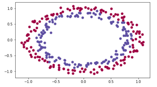
You would like a classifier to separate the blue dots from the red dots.

1 - Neural Network model

 

You will use a 3-layer neural network (already implemented for you). Here are the initialization methods you will experiment with:

• Zeros initialization -- setting initialization = "zeros" in the input argument.
• Random initialization -- setting initialization = "random" in the input argument. This initializes the weights to large random values.
• He initialization -- setting initialization = "he" in the input argument. This initializes the weights to random values scaled according to a paper by He et al., 2015.

Instructions: Please quickly read over the code below, and run it. In the next part you will implement the three initialization methods that this model() calls.

 【中文翻译】

1-神经网络模型

您将使用3层神经网络 (已经为您实施)。下面是您将要试验的初始化方法:

　　零初始化--在输入参数中设置initialization = "zeros"。

　　随机初始化--在输入参数中设置initialization = "random"。这会将权重初始化为大的随机值。

　　初始化-在输入参数中设置 initialization = "he"。这初始的权重随机值缩放根据一篇论文由He et al., 2015。

说明: 请快速阅读下面的代码, 并运行它。在下一部分中, 您将实现此 model() 调用的三初始化方法。

 【code】

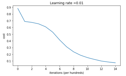
def model(X, Y, learning_rate = 0.01, num_iterations = 15000, print_cost = True, initialization = "he"):
    """
    Implements a three-layer neural network: LINEAR->RELU->LINEAR->RELU->LINEAR->SIGMOID.
    
    Arguments:
    X -- input data, of shape (2, number of examples)
    Y -- true "label" vector (containing 0 for red dots; 1 for blue dots), of shape (1, number of examples)
    learning_rate -- learning rate for gradient descent 
    num_iterations -- number of iterations to run gradient descent
    print_cost -- if True, print the cost every 1000 iterations
    initialization -- flag to choose which initialization to use ("zeros","random" or "he")
    
    Returns:
    parameters -- parameters learnt by the model
    """
        
    grads = {}
    costs = [] # to keep track of the loss
    m = X.shape[1] # number of examples
    layers_dims = [X.shape[0], 10, 5, 1]
    
    # Initialize parameters dictionary.
    if initialization == "zeros":
        parameters = initialize_parameters_zeros(layers_dims)
    elif initialization == "random":
        parameters = initialize_parameters_random(layers_dims)
    elif initialization == "he":
        parameters = initialize_parameters_he(layers_dims)

    # Loop (gradient descent)

    for i in range(0, num_iterations):

        # Forward propagation: LINEAR -> RELU -> LINEAR -> RELU -> LINEAR -> SIGMOID.
        a3, cache = forward_propagation(X, parameters)
        
        # Loss
        cost = compute_loss(a3, Y)

        # Backward propagation.
        grads = backward_propagation(X, Y, cache)
        
        # Update parameters.
        parameters = update_parameters(parameters, grads, learning_rate)
        
        # Print the loss every 1000 iterations
        if print_cost and i % 1000 == 0:
            print("Cost after iteration {}: {}".format(i, cost))
            costs.append(cost)
            
    # plot the loss
    plt.plot(costs)
    plt.ylabel('cost')
    plt.xlabel('iterations (per hundreds)')
    plt.title("Learning rate =" + str(learning_rate))
    plt.show()
    
    return parameters

2 - Zero initialization

There are two types of parameters to initialize in a neural network:

• the weight matrices (W^[1],W^[2],W^[3],...,W^[L−1],W^[L])
  
• the bias vectors (b^[1],b^[2],b^[3],...,b^[L−1],b^[L])
  

Exercise: Implement the following function to initialize all parameters to zeros. You'll see later that this does not work well since it fails to "break symmetry", but lets try it anyway and see what happens. Use np.zeros((..,..)) with the correct shapes.

【code】

# GRADED FUNCTION: initialize_parameters_zeros 

def initialize_parameters_zeros(layers_dims):
    """
    Arguments:
    layer_dims -- python array (list) containing the size of each layer.
    
    Returns:
    parameters -- python dictionary containing your parameters "W1", "b1", ..., "WL", "bL":
                    W1 -- weight matrix of shape (layers_dims[1], layers_dims[0])
                    b1 -- bias vector of shape (layers_dims[1], 1)
                    ...
                    WL -- weight matrix of shape (layers_dims[L], layers_dims[L-1])
                    bL -- bias vector of shape (layers_dims[L], 1)
    """
    
    parameters = {}
    L = len(layers_dims)            # number of layers in the network
    
    for l in range(1, L):
        ### START CODE HERE ### (≈ 2 lines of code)
        parameters['W' + str(l)] = np.zeros((layers_dims[l], layers_dims[l-1]))
        parameters['b' + str(l)] =  np.zeros((layers_dims[l],1))
        ### END CODE HERE ###
    return parameters

parameters = initialize_parameters_zeros([3,2,1])
print("W1 = " + str(parameters["W1"]))
print("b1 = " + str(parameters["b1"]))
print("W2 = " + str(parameters["W2"]))
print("b2 = " + str(parameters["b2"]))

【result】

W1 = [[ 0.  0.  0.]
 [ 0.  0.  0.]]
b1 = [[ 0.]
 [ 0.]]
W2 = [[ 0.  0.]]
b2 = [[ 0.]]

Expected Output:

W1	[[ 0. 0. 0.] [ 0. 0. 0.]]
b1	[[ 0.] [ 0.]]
W2	[[ 0. 0.]]
b2	[[ 0.]]

 Run the following code to train your model on 15,000 iterations using zeros initialization.

【code】

parameters = model(train_X, train_Y, initialization = "zeros")
print ("On the train set:")
predictions_train = predict(train_X, train_Y, parameters)
print ("On the test set:")
predictions_test = predict(test_X, test_Y, parameters)

【result】

Cost after iteration 0: 0.6931471805599453
Cost after iteration 1000: 0.6931471805599453
Cost after iteration 2000: 0.6931471805599453
Cost after iteration 3000: 0.6931471805599453
Cost after iteration 4000: 0.6931471805599453
Cost after iteration 5000: 0.6931471805599453
Cost after iteration 6000: 0.6931471805599453
Cost after iteration 7000: 0.6931471805599453
Cost after iteration 8000: 0.6931471805599453
Cost after iteration 9000: 0.6931471805599453
Cost after iteration 10000: 0.6931471805599455
Cost after iteration 11000: 0.6931471805599453
Cost after iteration 12000: 0.6931471805599453
Cost after iteration 13000: 0.6931471805599453
Cost after iteration 14000: 0.6931471805599453

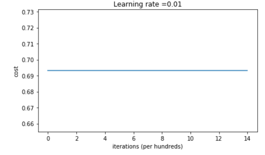
On the train set:
Accuracy: 0.5
On the test set:
Accuracy: 0.5

The performance is really bad, and the cost does not really decrease, and the algorithm performs no better than random guessing. Why? Lets look at the details of the predictions and the decision boundary:

 【中文翻译】

性能真的很差, 成本函数并没有真正减少, 算法的执行效果不比随机猜测好。为什么?让我们看一下预测和决策边界的细节:

【code】

print ("predictions_train = " + str(predictions_train))
print ("predictions_test = " + str(predictions_test))

【】result 

predictions_train = [[0 0 0 0 0 0 0 0 0 0 0 0 0 0 0 0 0 0 0 0 0 0 0 0 0 0 0 0 0 0 0 0 0 0 0 0 0
  0 0 0 0 0 0 0 0 0 0 0 0 0 0 0 0 0 0 0 0 0 0 0 0 0 0 0 0 0 0 0 0 0 0 0 0 0
  0 0 0 0 0 0 0 0 0 0 0 0 0 0 0 0 0 0 0 0 0 0 0 0 0 0 0 0 0 0 0 0 0 0 0 0 0
  0 0 0 0 0 0 0 0 0 0 0 0 0 0 0 0 0 0 0 0 0 0 0 0 0 0 0 0 0 0 0 0 0 0 0 0 0
  0 0 0 0 0 0 0 0 0 0 0 0 0 0 0 0 0 0 0 0 0 0 0 0 0 0 0 0 0 0 0 0 0 0 0 0 0
  0 0 0 0 0 0 0 0 0 0 0 0 0 0 0 0 0 0 0 0 0 0 0 0 0 0 0 0 0 0 0 0 0 0 0 0 0
  0 0 0 0 0 0 0 0 0 0 0 0 0 0 0 0 0 0 0 0 0 0 0 0 0 0 0 0 0 0 0 0 0 0 0 0 0
  0 0 0 0 0 0 0 0 0 0 0 0 0 0 0 0 0 0 0 0 0 0 0 0 0 0 0 0 0 0 0 0 0 0 0 0 0
  0 0 0 0]]
predictions_test = [[0 0 0 0 0 0 0 0 0 0 0 0 0 0 0 0 0 0 0 0 0 0 0 0 0 0 0 0 0 0 0 0 0 0 0 0 0
  0 0 0 0 0 0 0 0 0 0 0 0 0 0 0 0 0 0 0 0 0 0 0 0 0 0 0 0 0 0 0 0 0 0 0 0 0
  0 0 0 0 0 0 0 0 0 0 0 0 0 0 0 0 0 0 0 0 0 0 0 0 0 0]]

 【code】

plt.title("Model with Zeros initialization")
axes = plt.gca()
axes.set_xlim([-1.5,1.5])
axes.set_ylim([-1.5,1.5])
plot_decision_boundary(lambda x: predict_dec(parameters, x.T), train_X, train_Y)

【result】

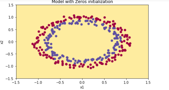
The model is predicting 0 for every example.

In general, initializing all the weights to zero results in the network failing to break symmetry. This means that every neuron in each layer will learn the same thing, and you might as well be training a neural network with n^[l]=1 for every layer, and the network is no more powerful than a linear classifier such as logistic regression.

 

What you should remember:

• The weights W[l]W[l] should be initialized randomly to break symmetry.
• It is however okay to initialize the biases b^[l] to zeros. Symmetry is still broken so long as W^[l] is initialized randomly.

3 - Random initialization

To break symmetry, lets intialize the weights randomly. Following random initialization, each neuron can then proceed to learn a different function of its inputs. In this exercise, you will see what happens if the weights are intialized randomly, but to very large values.

Exercise: Implement the following function to initialize your weights to large random values (scaled by *10) and your biases to zeros. Use np.random.randn(..,..) * 10 for weights and np.zeros((.., ..)) for biases. We are using a fixed np.random.seed(..) to make sure your "random" weights match ours, so don't worry if running several times your code gives you always the same initial values for the parameters.

【code】

# GRADED FUNCTION: initialize_parameters_random

def initialize_parameters_random(layers_dims):
    """
    Arguments:
    layer_dims -- python array (list) containing the size of each layer.
    
    Returns:
    parameters -- python dictionary containing your parameters "W1", "b1", ..., "WL", "bL":
                    W1 -- weight matrix of shape (layers_dims[1], layers_dims[0])
                    b1 -- bias vector of shape (layers_dims[1], 1)
                    ...
                    WL -- weight matrix of shape (layers_dims[L], layers_dims[L-1])
                    bL -- bias vector of shape (layers_dims[L], 1)
    """
    
    np.random.seed(3)               # This seed makes sure your "random" numbers will be the as ours
    parameters = {}
    L = len(layers_dims)            # integer representing the number of layers
    
    for l in range(1, L):
        ### START CODE HERE ### (≈ 2 lines of code)
        parameters['W' + str(l)] = np.random.randn(layers_dims[l], layers_dims[l-1]) * 10
        parameters['b' + str(l)] = np.zeros((layers_dims[l], 1))
        ### END CODE HERE ###

    return parameters

parameters = initialize_parameters_random([3, 2, 1])
print("W1 = " + str(parameters["W1"]))
print("b1 = " + str(parameters["b1"]))
print("W2 = " + str(parameters["W2"]))
print("b2 = " + str(parameters["b2"]))

【result】

W1 = [[ 17.88628473   4.36509851   0.96497468]
 [-18.63492703  -2.77388203  -3.54758979]]
b1 = [[ 0.]
 [ 0.]]
W2 = [[-0.82741481 -6.27000677]]
b2 = [[ 0.]]

Expected Output:

W1	[[ 17.88628473 4.36509851 0.96497468] [-18.63492703 -2.77388203 -3.54758979]]
b1	[[ 0.] [ 0.]]
W2	[[-0.82741481 -6.27000677]]
b2	[[ 0.]]

Run the following code to train your model on 15,000 iterations using random initialization.

【code】

parameters = model(train_X, train_Y, initialization = "random")
print ("On the train set:")
predictions_train = predict(train_X, train_Y, parameters)
print ("On the test set:")
predictions_test = predict(test_X, test_Y, parameters)

【result】

Cost after iteration 0: inf
Cost after iteration 1000: 0.6237287551108738
Cost after iteration 2000: 0.5981106708339466
Cost after iteration 3000: 0.5638353726276827
Cost after iteration 4000: 0.550152614449184
Cost after iteration 5000: 0.5444235275228304
Cost after iteration 6000: 0.5374184054630083
Cost after iteration 7000: 0.47357131493578297
Cost after iteration 8000: 0.39775634899580387
Cost after iteration 9000: 0.3934632865981078
Cost after iteration 10000: 0.39202525076484457
Cost after iteration 11000: 0.38921493051297673
Cost after iteration 12000: 0.38614221789840486
Cost after iteration 13000: 0.38497849983013926
Cost after iteration 14000: 0.38278397192120406

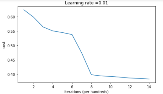
On the train set:
Accuracy: 0.83
On the test set:
Accuracy: 0.86

If you see "inf" as the cost after the iteration 0, this is because of numerical roundoff(数字的舍入); a more numerically sophisticated implementation （更复杂的实现）would fix this. But this isn't worth worrying about for our purposes.

Anyway, it looks like you have broken symmetry, and this gives better results. than before. The model is no longer outputting all 0s.

【code】

print (predictions_train)
print (predictions_test)

【result】

[[1 0 1 1 0 0 1 1 1 1 1 0 1 0 0 1 0 1 1 0 0 0 1 0 1 1 1 1 1 1 0 1 1 0 0 1 1
  1 1 1 1 1 1 0 1 1 1 1 0 1 0 1 1 1 1 0 0 1 1 1 1 0 1 1 0 1 0 1 1 1 1 0 0 0
  0 0 1 0 1 0 1 1 1 0 0 1 1 1 1 1 1 0 0 1 1 1 0 1 1 0 1 0 1 1 0 1 1 0 1 0 1
  1 0 0 1 0 0 1 1 0 1 1 1 0 1 0 0 1 0 1 1 1 1 1 1 1 0 1 1 0 0 1 1 0 0 0 1 0
  1 0 1 0 1 1 1 0 0 1 1 1 1 0 1 1 0 1 0 1 1 0 1 0 1 1 1 1 0 1 1 1 1 0 1 0 1
  0 1 1 1 1 0 1 1 0 1 1 0 1 1 0 1 0 1 1 1 0 1 1 1 0 1 0 1 0 0 1 0 1 1 0 1 1
  0 1 1 0 1 1 1 0 1 1 1 1 0 1 0 0 1 1 0 1 1 1 0 0 0 1 1 0 1 1 1 1 0 1 1 0 1
  1 1 0 0 1 0 0 0 1 0 0 0 1 1 1 1 0 0 0 0 1 1 1 1 0 0 1 1 1 1 1 1 1 0 0 0 1
  1 1 1 0]]
[[1 1 1 1 0 1 0 1 1 0 1 1 1 0 0 0 0 1 0 1 0 0 1 0 1 0 1 1 1 1 1 0 0 0 0 1 0
  1 1 0 0 1 1 1 1 1 0 1 1 1 0 1 0 1 1 0 1 0 1 0 1 1 1 1 1 1 1 1 1 0 1 0 1 1
  1 1 1 0 1 0 0 1 0 0 0 1 1 0 1 1 0 0 0 1 1 0 1 1 0 0]]

【code】

plt.title("Model with large random initialization")
axes = plt.gca()
axes.set_xlim([-1.5,1.5])
axes.set_ylim([-1.5,1.5])
plot_decision_boundary(lambda x: predict_dec(parameters, x.T), train_X, train_Y)

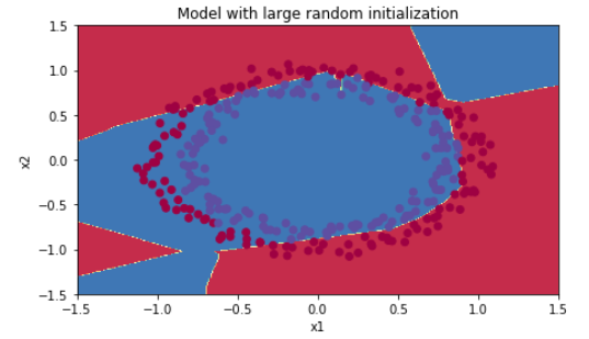
Observations:

• The cost starts very high. This is because with large random-valued weights, the last activation (sigmoid) outputs results that are very close to 0 or 1 for some examples, and when it gets that example wrong it incurs a very high loss for that example. Indeed, when log(a[3])=log(0)log⁡(a[3])=log⁡(0), the loss goes to infinity.
• Poor initialization can lead to vanishing/exploding gradients, which also slows down the optimization algorithm.
• If you train this network longer you will see better results, but initializing with overly large random numbers slows down the optimization.

In summary:

• Initializing weights to very large random values does not work well.
• Hopefully intializing with small random values does better. The important question is: how small should be these random values be? Lets find out in the next part!

4 - He initialization

Finally, try "He Initialization"; this is named for the first author of He et al., 2015. (If you have heard of "Xavier initialization", this is similar except Xavier initialization uses a scaling factor for the weights W[l]W[l] of sqrt(1./layers_dims[l-1]) where He initialization would use sqrt(2./layers_dims[l-1]).)

Exercise: Implement the following function to initialize your parameters with He initialization.

Hint: This function is similar to the previous initialize_parameters_random(...). The only difference is that instead of multiplying np.random.randn(..,..) by 10, you will multiply it by 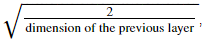 which is what He initialization recommends for layers with a ReLU activation.

 【code】

# GRADED FUNCTION: initialize_parameters_he

def initialize_parameters_he(layers_dims):
    """
    Arguments:
    layer_dims -- python array (list) containing the size of each layer.
    
    Returns:
    parameters -- python dictionary containing your parameters "W1", "b1", ..., "WL", "bL":
                    W1 -- weight matrix of shape (layers_dims[1], layers_dims[0])
                    b1 -- bias vector of shape (layers_dims[1], 1)
                    ...
                    WL -- weight matrix of shape (layers_dims[L], layers_dims[L-1])
                    bL -- bias vector of shape (layers_dims[L], 1)
    """
    
    np.random.seed(3)
    parameters = {}
    L = len(layers_dims) - 1 # integer representing the number of layers
     
    for l in range(1, L + 1):
        ### START CODE HERE ### (≈ 2 lines of code)
        parameters['W' + str(l)] =  np.random.randn(layers_dims[l], layers_dims[l-1]) * np.sqrt(2./layers_dims[l-1])
        parameters['b' + str(l)] = np.zeros((layers_dims[l],1))
        ### END CODE HERE ###
        
    return parameters

parameters = initialize_parameters_he([2, 4, 1])
print("W1 = " + str(parameters["W1"]))
print("b1 = " + str(parameters["b1"]))
print("W2 = " + str(parameters["W2"]))
print("b2 = " + str(parameters["b2"]))

【result】

W1 = [[ 1.78862847  0.43650985]
 [ 0.09649747 -1.8634927 ]
 [-0.2773882  -0.35475898]
 [-0.08274148 -0.62700068]]
b1 = [[ 0.]
 [ 0.]
 [ 0.]
 [ 0.]]
W2 = [[-0.03098412 -0.33744411 -0.92904268  0.62552248]]
b2 = [[ 0.]]

Expected Output:

W1	[[ 1.78862847 0.43650985] [ 0.09649747 -1.8634927 ] [-0.2773882 -0.35475898] [-0.08274148 -0.62700068]]
b1	[[ 0.] [ 0.] [ 0.] [ 0.]]
W2	[[-0.03098412 -0.33744411 -0.92904268 0.62552248]]
b2	[[ 0.]]

 Run the following code to train your model on 15,000 iterations using He initialization.

【code】 

parameters = model(train_X, train_Y, initialization = "he")
print ("On the train set:")
predictions_train = predict(train_X, train_Y, parameters)
print ("On the test set:")
predictions_test = predict(test_X, test_Y, parameters)

 【reuslt】

Cost after iteration 0: 0.8830537463419761
Cost after iteration 1000: 0.6879825919728063
Cost after iteration 2000: 0.6751286264523371
Cost after iteration 3000: 0.6526117768893807
Cost after iteration 4000: 0.6082958970572938
Cost after iteration 5000: 0.5304944491717495
Cost after iteration 6000: 0.4138645817071794
Cost after iteration 7000: 0.3117803464844441
Cost after iteration 8000: 0.23696215330322562
Cost after iteration 9000: 0.18597287209206836
Cost after iteration 10000: 0.1501555628037182
Cost after iteration 11000: 0.12325079292273548
Cost after iteration 12000: 0.09917746546525937
Cost after iteration 13000: 0.0845705595402428
Cost after iteration 14000: 0.07357895962677366

On the train set:
Accuracy: 0.993333333333
On the test set:
Accuracy: 0.96

【code】

plt.title("Model with He initialization")
axes = plt.gca()
axes.set_xlim([-1.5,1.5])
axes.set_ylim([-1.5,1.5])
plot_decision_boundary(lambda x: predict_dec(parameters, x.T), train_X, train_Y)

Observations:

• The model with He initialization separates the blue and the red dots very well in a small number of iterations.

5 - Conclusions

 

You have seen three different types of initializations. For the same number of iterations and same hyperparameters the comparison is:

Model	Train accuracy	Problem/Comment
3-layer NN with zeros initialization	50%	fails to break symmetry
3-layer NN with large random initialization	83%	too large weights
3-layer NN with He initialization	99%	recommended method

What you should remember from this notebook:

• Different initializations lead to different results
• Random initialization is used to break symmetry and make sure different hidden units can learn different things
• Don't intialize to values that are too large
• He initialization works well for networks with ReLU activations.