Notes - Berkerly Statistics 2.1X - Week2
-Week2, 2014/03/06, hphp
欢迎交流、转载,转载请注明出处~
Week2. Location , Represents of data
Summarizing data can help us understand them, especially when the number of data is large. This chapter presents several ways to summarize quantitative data by a typical value(a measure of location, such as the mean, median, or mode) and a measure of how well the typical value represents the list (a measure of spread, such as the range, inter-quartile range, or standard deviation). Markov's and Chebychev's inequalities show that these summary measures can contain a surprisingly large amount of information about the data.
Lecture 3.1 The median and the mode
Measures of location
Measures of location do just that: They try to capture with a single number what is typical of the data.
Mean , Median , Mode.
Median:The median is the number that divides the (ordered) data in half—thesmallestnumber that is at least as big as half the data. At least half the data are equal to or smaller than the median, and at least half the data are equal to or greater than the median.
EG.list:1, 2, 3, 4
median: -- > 2
1/4 th: -- > 1
3/4 th: -- > 3
However, the mean, the median, and the mode are "as close as possible" to all the data: Foreach of these three measures of location, the sum of the distances between each datum and the measure of location is as small as it can be. The differences among the three measures of location are in how "distance" is defined.[1]
The mean, median, and mode can berelated (approximately) to the histogram: loosely speaking, the mode is the highest bump, the median is where half the area is to the right and half is to the left, and the mean is where the histogram would balance, were it a solid object cut out of a uniform block of metal. (All these heuristics are approximate, and depend on the class intervals.)
[datum : 数据]
[Symmetric Distribution - average , balanced.]
The center
Median : the "half point" of the data" --- > 31.4 mm
The Mode: The "most common" value
the value has the highest frequency
4 | 8
5 | 9
6 |3337
7 |000235
8 | 012345788
9 | 015556
10| 0
6|333
7|000
9|555
A unimodal distribution
Unimodal : one peak
Lecture 3.2 The average
average - mean
The average - not center , not even a member , not variable members.
not so many difference with what i have already understood.
Lecture 3.3 Comparing and combining averages
What's the relation between these groups

[Natinal Health and Nutrition Examination 1999-2000] [noting the data and the source.]
the data are not longitudinal, but are cross sectional.
Comparing the numbers
- the average of diff groups :"how are the groups related to each other"
E.G.
ave section1 60 section2 70 cant tell the average , because the lack of information.
ave section size section1 60 20 section2 70 30
average = total/50
- weighted average of averages
ave section size section proportion section1 60 20 2/5 section2 70 30 3/5 average = 60*2/5 + 70*3/5
average = SUM(average[i]*weigth[i]) [weights are the section proportions.]
Lecture 3.4 The average and the histogram; The average and the median.
the median is unaffected by outliers.
[ Statistics that are not affected too much by small subsets of the data are resistant. The median is resistant; the mean is not. ]
A right-skewed distribution : average is greater than the median.
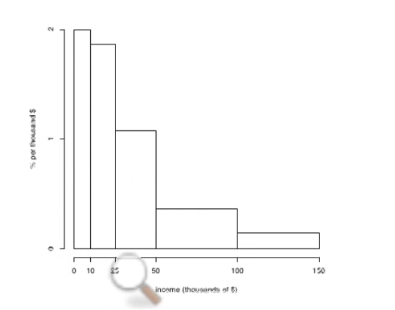
incomes
[affluent-rich,enrich]
[gizmos and gadget-创意和配件]
[disingenuously - 狡猾]
[pledge to - 承诺]
[Articles report median incomes. instead of average income.]
What does an average test score tell u.
- if a lot of people did not get good scores , the histogram will get : Left-hand tail.
The average and the histogram
- list : 2, 3, 3, 4
average = [ (1*2) + (2*3) + (1*4) ]/4 = 1/4*2 + 2/4*3 + 1/4*4
1/4,2/4,1/4 --> the percent/ proportions..
- list : 2, 3, 3, 7
average = [ (1*2) + (2*3) + (1*4) ]/4 = 1/4*2 + 2/4*3 + 1/4*4
1/4,2/4,1/4 --> the percent/ proportions..
- the average is the center of gravity of the histogram
1/4,2/4,1/4:weights
Lecture 3.5 Markov's inequality
How far can u be above average , How big can the tail be
- Andrey Markov(1856-1922)
- The average of a group people is 20years, What proportion are more than 80 years old.
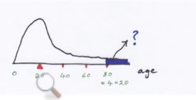
- Markov's inequality:
If a list has only non-negative entries , then the proportion of entries are at least at large as k times the average is at most 1/k.
[could use the Sum( weight*value ) as a prove.]
- taking care of the edge
Question: more than 80 years old: > 80
Markov: more than or equal 80 years old : >= 80
- But , if k = 0.5 , the biggest proportion will be 200% , makes no sense though.
Lecture 4.1 How the average/other represents data
Measures of location summarize what is typical of elements of a list, but not every element is typical. Are all the elements close to each other? Are most of the elements close to each other? What is the biggest difference between elements? On the average, how far are the elements from each other? Measures of spread or variability tell us.
The three most common measures of spreador variability are the range, theinterquartile range (IQR), and thestandard deviation (SD).
The range of a list is the largest value minus the smallest value.
It is the width of the smallest interval that contains all the data, so it measures spread. It is notresistant, because changing just one datum can make it arbitrarily large.Range and interquartile range.
- How far are these data from the center.
- Spread
- IQR : Inter quartile range

The middle 50% data are spread over 8 years.
Lecture 4.2 Standard Deviation
Deviation from average: roughly how far are the numbers from their average?
- list : 2, 3, 3, 4, 4, 5, 6, 7 average = 4.25
- deviations: 2.25, 1.25, 1.25, 0.25, 0.25, -0.75, -1.75, -2.75 ---> the average of deviations is 0.
- BUT absolute values does not have good math properties.
Standard Deviation
- Root mean square of deviation from the average --- Rms????
The rms (root mean square) of a list measures the average size of its entries. It is defined as follows:
rms = square-root( (sum of the squares of the entries)/(number of entries) )
=[ (sum of squares of the entries)/(number of entries) ]½.
- How does the sd are measured or representitive for a list of data ?
$List: 2, 3, 3, 4, 4, 5, 6, 7 average = 4.25
variance = mean square of deviation from the average
SD = root 2.44 = 1.56 $
The average and sd use the same units.
---> SD is the measure spread of the data.
the measure spread of the data
- The interval average +- SD is roughly [2.75, 5.75]
- It picks up a good chunk of the list, but not all.

Lecture 4.3 Properties of the SD:Chebychev's inequality
In a nutshell
Rough statement : No matter what the list , tha vast majority of entries will be in the range average +- a_few_SDs.
- Chebycheff(19 centry)
- Chebycheff's inequality:
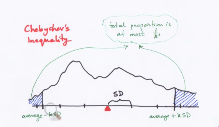
- Precise statement:
No mater what the list , a proportion of at least 1-1/k^2 of the entries will be in the range average +/- k*SD
Prove
Instinctly , if the proportion of data that > average + k*SD are bigger than 1/k^2, than , the SD will get larger.
FootPrints
[1]. meaning of distances for "Mean, Median, Mode":
For the mean, the distance between two numbers is defined to be the square of their difference.
That is, the sum of the squares of the differences between the data and the mean is smaller than the sum of squares of the differences between the data and any other number. (Equivalently, the rms or root mean square of the differences from the mean is smaller than the rms of the list of differences from any other number—the rms is defined and discussed below.)
For the median, the distance between two numbers is defined to be the absolute value of their difference. That is, the sum of the absolute values of the differences between a median and the data is no larger than the sum of the absolute values of the differences between any other number and the data.
For the mode, the distance between two numbers is defined to be zero if the numbers are equal, and one if they are not equal. That is, the number of data that differ from a mode is no larger than the number of data that differ from any other value. Equivalently, a mode is a number from which the fewest possible data differ: a "most common" value.