机器学习算法及代码实现–支持向量机

机器学习算法及代码实现–支持向量机

1、支持向量机

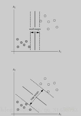
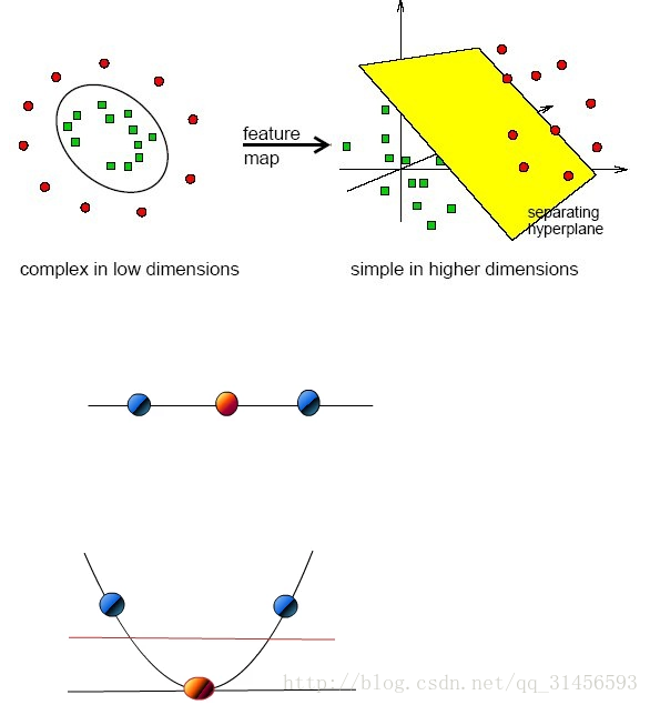
SVM希望通过N-1维的分隔超平面线性分开N维的数据，距离分隔超平面最近的点被叫做支持向量，我们利用SMO（SVM实现方法之一）最大化支持向量到分隔面的距离，这样当新样本点进来时，其被分类正确的概率也就更大。我们计算样本点到分隔超平面的函数间隔，如果函数间隔为正，则分类正确，函数间隔为负，则分类错误，函数间隔的绝对值除以||w||就是几何间隔，几何间隔始终为正，可以理解为样本点到分隔超平面的几何距离。若数据不是线性可分的，那我们引入核函数的概念，从某个特征空间到另一个特征空间的映射是通过核函数来实现的，我们利用核函数将数据从低维空间映射到高维空间，低维空间的非线性问题在高维空间往往会成为线性问题，再利用N-1维分割超平面对数据分类。

2、分类

线性可分、线性不可分

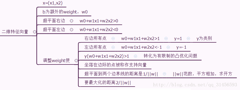
3、超平面公式（先考虑线性可分）

W*X+b=0
其中W={w1,w2,,,w3}，为权重向量
下面用简单的二维向量讲解（思维导图）

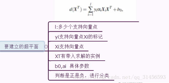
4、寻找超平面

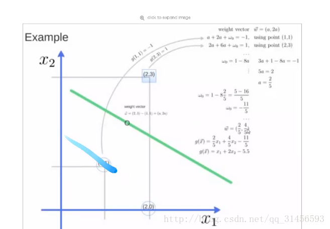
5、例子

6、线性不可分

映射到高维

算法思路（思维导图）

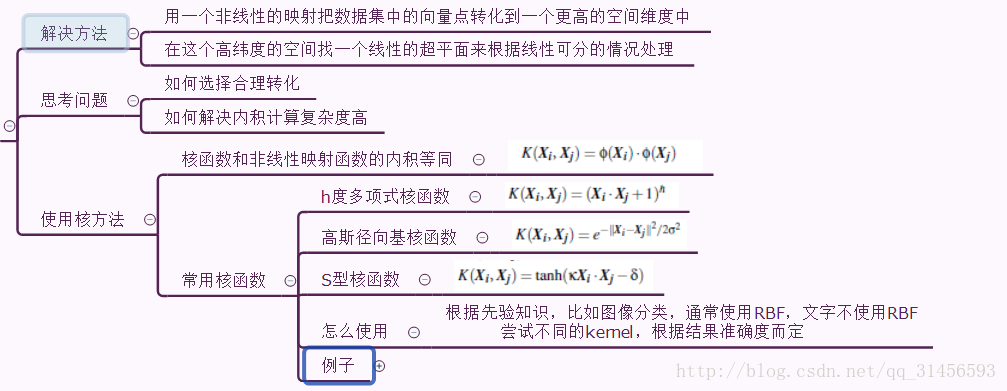
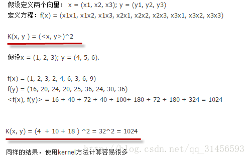
核函数举例

代码

# -*- coding: utf-8 -*-
from sklearn import svm

# 数据
x = [[2, 0], [1, 1], [2, 3]]
# 标签
y = [0, 0, 1]
# 线性可分的svm分类器，用线性的核函数
clf = svm.SVC(kernel='linear')
# 训练
clf.fit(x, y)
print clf

# 获得支持向量
print clf.support_vectors_

# 获得支持向量点在原数据中的下标
print clf.support_

# 获得每个类支持向量的个数
print clf.n_support_

# 预测
print clf.predict([2, 0])

# -*- coding: utf-8 -*-
import numpy as np
import pylab as pl
from sklearn import svm

np.random.seed(0)  # 值固定，每次随机结果不变
# 2组20个二维的随机数，20个0，20个1的y  （20，2）20行2列
X = np.r_[np.random.randn(20, 2) - [2, 2], np.random.randn(20, 2) + [2, 2]]
Y = [0] * 20 + [1] * 20

# 训练
clf = svm.SVC(kernel='linear')
clf.fit(X, Y)


w = clf.coef_[0]
a = -w[0] / w[1]
xx = np.linspace(-5, 5)
yy = a * xx - (clf.intercept_[0] / w[1])  # 点斜式 平分的线


b = clf.support_vectors_[0]
yy_down = a* xx +(b[1] - a*b[0])
b = clf.support_vectors_[-1]
yy_up = a* xx +(b[1] - a*b[0])  # 两条虚线

print "w: ", w
print "a: ", a
# print " xx: ", xx
# print " yy: ", yy
print "support_vectors_: ", clf.support_vectors_
print "clf.coef_: ", clf.coef_

# In scikit-learn coef_ attribute holds the vectors of the separating hyperplanes for linear models. It has shape (n_classes, n_features) if n_classes > 1 (multi-class one-vs-all) and (1, n_features) for binary classification.
#
# In this toy binary classification example, n_features == 2, hence w = coef_[0] is the vector orthogonal to the hyperplane (the hyperplane is fully defined by it + the intercept).
#
# To plot this hyperplane in the 2D case (any hyperplane of a 2D plane is a 1D line), we want to find a f as in y = f(x) = a.x + b. In this case a is the slope of the line and can be computed by a = -w[0] / w[1].




# plot the line, the points, and the nearest vectors to the plane
pl.plot(xx, yy, 'k-')
pl.plot(xx, yy_down, 'k--')
pl.plot(xx, yy_up, 'k--')

pl.scatter(clf.support_vectors_[:, 0], clf.support_vectors_[:, 1],
           s=80, facecolors='none')
pl.scatter(X[:, 0], X[:, 1], c=Y, cmap=pl.cm.Paired)

pl.axis('tight')
pl.show()

# -*- coding: utf-8 -*-
from __future__ import print_function

from time import time
import logging  # 打印程序进展的信息
import matplotlib.pyplot as plt

from sklearn.cross_validation import train_test_split
from sklearn.datasets import fetch_lfw_people
from sklearn.grid_search import GridSearchCV
from sklearn.metrics import classification_report
from sklearn.metrics import confusion_matrix
from sklearn.decomposition import RandomizedPCA
from sklearn.svm import SVC


print(__doc__)

# 打印程序进展的信息
logging.basicConfig(level=logging.INFO, format='%(asctime)s %(message)s')


###############################################################################
# 下载人脸数据集,并导入

lfw_people = fetch_lfw_people(min_faces_per_person=70, resize=0.4)

# 数据集多少，长宽多少
n_samples, h, w = lfw_people.images.shape

# x是特征向量的矩阵，获取矩阵列数，即纬度
X = lfw_people.data
n_features = X.shape[1]

# y是分类标签向量
y = lfw_people.target
# 类别里面有谁的名字
target_names = lfw_people.target_names
# 名字有多少行，即有多少人要区分
n_classes = target_names.shape[0]

# 打印
print("Total dataset size:")
print("n_samples: %d" % n_samples)
print("n_features: %d" % n_features)
print("n_classes: %d" % n_classes)


###############################################################################
# 将数据集划分为训练集和测试集，测试集占0.25
X_train, X_test, y_train, y_test = train_test_split(
    X, y, test_size=0.25)


###############################################################################
# PCA降维
n_components = 150  # 组成元素数量

print("Extracting the top %d eigenfaces from %d faces"
      % (n_components, X_train.shape[0]))
t0 = time()
# 建立PCA模型
pca = RandomizedPCA(n_components=n_components, whiten=True).fit(X_train)
print("done in %0.3fs" % (time() - t0))

# 提取特征脸
eigenfaces = pca.components_.reshape((n_components, h, w))

print("Projecting the input data on the eigenfaces orthonormal basis")
t0 = time()
# 将特征向量转化为低维矩阵
X_train_pca = pca.transform(X_train)
X_test_pca = pca.transform(X_test)
print("done in %0.3fs" % (time() - t0))


###############################################################################
# Train a SVM classification model

print("Fitting the classifier to the training set")
t0 = time()
# C错误惩罚权重 gamma 建立核函数的不同比例
param_grid = {'C': [1e3, 5e3, 1e4, 5e4, 1e5],
              'gamma': [0.0001, 0.0005, 0.001, 0.005, 0.01, 0.1], }
# 选择核函数，建SVC，尝试运行，获得最好参数
clf = GridSearchCV(SVC(kernel='rbf', class_weight='auto'), param_grid)
# 训练
clf = clf.fit(X_train_pca, y_train)
print("done in %0.3fs" % (time() - t0))
print("Best estimator found by grid search:")
print(clf.best_estimator_)  # 输出最佳参数


###############################################################################
# Quantitative evaluation of the model quality on the test set

print("Predicting people's names on the test set")
t0 = time()
# 预测
y_pred = clf.predict(X_test_pca)
print("done in %0.3fs" % (time() - t0))

print(classification_report(y_test, y_pred, target_names=target_names))  # 与真实情况作对比求置信度
print(confusion_matrix(y_test, y_pred, labels=range(n_classes)))  # 对角线的为预测正确的，a预测为a


###############################################################################
# Qualitative evaluation of the predictions using matplotlib

def plot_gallery(images, titles, h, w, n_row=3, n_col=4):
    """Helper function to plot a gallery of portraits"""
    plt.figure(figsize=(1.8 * n_col, 2.4 * n_row))
    plt.subplots_adjust(bottom=0, left=.01, right=.99, top=.90, hspace=.35)
    for i in range(n_row * n_col):
        plt.subplot(n_row, n_col, i + 1)
        plt.imshow(images[i].reshape((h, w)), cmap=plt.cm.gray)
        plt.title(titles[i], size=12)
        plt.xticks(())
        plt.yticks(())


# plot the result of the prediction on a portion of the test set

def title(y_pred, y_test, target_names, i):
    pred_name = target_names[y_pred[i]].rsplit(' ', 1)[-1]
    true_name = target_names[y_test[i]].rsplit(' ', 1)[-1]
    return 'predicted: %s
true:      %s' % (pred_name, true_name)

prediction_titles = [title(y_pred, y_test, target_names, i)
                     for i in range(y_pred.shape[0])]

plot_gallery(X_test, prediction_titles, h, w)  # 画出测试集和它的title

# plot the gallery of the most significative eigenfaces

eigenface_titles = ["eigenface %d" % i for i in range(eigenfaces.shape[0])]
plot_gallery(eigenfaces, eigenface_titles, h, w)  # 打印特征脸

plt.show()  # 显示