再进行Mini-batch 梯度下降法学习之前,我们首先对梯度下降法进行理解
一、梯度下降法(Gradient Descent)
优化思想:用当前位置的负梯度方向作为搜索方向,亦即为当前位置下降最快的方向,也称“最速下降法”。越接近目标值时,步长越小,下降越慢。
首先来看看梯度下降的一个直观的解释。比如我们在一座大山上的某处位置,由于我们不知道怎么下山,于是决定走一步算一步,也就是在每走到一个位置的时候,求解当前位置的梯度,沿着梯度的负方向,也就是当前最陡峭的位置向下走一步,然后继续求解当前位置梯度,向这一步所在位置沿着最陡峭最易下山的位置走一步。这样一步步的走下去,一直走到觉得我们已经到了山脚。当然这样走下去,有可能我们不能走到山脚,而是到了某一个局部的山峰低处。
从上面的解释可以看出,梯度下降不一定能够找到全局的最优解,有可能是一个局部最优解。当然,如果损失函数是凸函数,梯度下降法得到的解就一定是全局最优解。

接下来我们了解一下梯度下降法的相关概念
二、批量梯度下降法(Batch Gradient Descent,BGD)
在更新参数时,BGD根据batch中的所有样本对参数进行更新。

三、随机梯度下降法(Stochastic Gradient Descent,SGD)
随机梯度下降法,其实和批量梯度下降法原理类似,区别在与求梯度时没有用所有的m个样本的数据,而是仅仅选取一个样本j来求梯度。对应的更新公式是:

随机梯度下降法,和批量梯度下降法是两个极端,一个采用所有数据来梯度下降,一个用一个样本来梯度下降。自然各自的优缺点都非常突出。对于训练速度来说,随机梯度下降法由于每次仅仅采用一个样本来迭代,训练速度很快,而批量梯度下降法在样本量很大的时候,训练速度不能让人满意。对于准确度来说,随机梯度下降法用于仅仅用一个样本决定梯度方向,导致解很有可能不是最优。对于收敛速度来说,由于随机梯度下降法一次迭代一个样本,导致迭代方向变化很大,不能很快的收敛到局部最优解。
四、小批量梯度下降法(Mini-batch Gradient Descent)——>重点
小批量梯度下降法是批量梯度下降法和随机梯度下降法的折衷,也就是对于m个样本,我们采用x个样子来迭代,1<x<m。一般可以取x=10,当然根据样本的数据,可以调整这个x的值。对应的更新公式是:
 五、三种方法代码演示
(一)准备工作
1、导入相关的包
import numpy as np
import os
#画图
%matplotlib inline
import matplotlib.pyplot as plt
2、保存图像
#保存图像
PROJECT_ROOT_DIR = "."
MODEL_ID = "linear_models"
3、生成随机种子
np.random.seed(42)
4、定义一个保存图像的函数
#定义一个保存图像的函数
def save_fig(fig_id,tight_layout=True):
    path = os.path.join(PROJECT_ROOT_DIR,"images",MODEL_ID,fig_id + ".png")#指定保存图像的路径
    print("Saving figure",fig_id)#提示函数,正在保存图片
    plt.savefig(path,format="png",dpi=300)#保存图片(需要指定保存路径,保存格式,清晰度)
5、过滤掉讨厌的警告信息
#过滤掉讨厌的警告信息
import warnings
warnings.filterwarnings(action="ignore",message="internal gelsd")
6、定义变量
#定义变量
import numpy as np

x = 2 * np.random.rand(100,1) #生成训练数据(特征部分)
y = 4 + 3 * x + np.random.randn(100,1) #生成训练数据(标签部分)
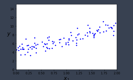
7、画出图像
#画出图像
plt.plot(x,y,"b.") #画图
plt.xlabel("$x_1$",fontsize=18)
plt.ylabel("$y$",fontsize=18,rotation=0)
plt.axis([0,2,0,15])
save_fig("generated_data_plot") #保存图片
plt.show()
8、添加新特征
#添加新特征
x_b = np.c_[np.ones((100,1)),x]
9、创建测试数据
#创建测试数据
x_new = np.array([[0],[2]])
x_new_b = np.c_[np.ones((2,1)),x_new]

#从sklearn包里导入线性回归模型
from sklearn.linear_model import LinearRegression
line_reg = LinearRegression() #创建线性回归对象
line_reg.fit(x,y) #拟合训练数据
line_reg.intercept_,line_reg.coef_  #输出截距,斜率
(array([4.21509616]), array([[2.77011339]]))
10、对测试集进行预测
#对测试集进行预测
line_reg.predict(x_new)
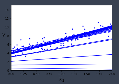
(二)用批量梯度下降求解线性回归
#用批量梯度下降求解线性回归
eta = 0.1
n_iterations = 100   #迭代次数
m =100
theta = np.random.randn(2,1)

for iteration in range(n_iterations):
    # h theta (x(i)) = x_b.dot(theta)

    gradients = 2/m * x_b.T.dot(x_b.dot(theta) - y )
    theta = theta - eta * gradients
m = len(x_b)
theta_path_bgd = []
def plot_gradient_descent(theta,eta,theta_path = None):
    m = len(x_b)
    plt.plot(x,y,"b.")
    n_iterations = 1000
    for iteration in range(n_iterations):
        if iteration <10:
            y_predict = x_new_b.dot(theta)
            style = "b-"
            plt.plot(x_new,y_predict,style)
        gradients = 2/m * x_b.T.dot(x_b.dot(theta) - y)
        theta = theta - eta *gradients
        if theta_path is not None:
            theta_path.append(theta)
    plt.xlabel("$x_1$",fontsize=18)
    plt.axis([0,2,0,15]) #坐标,横坐标0-2,纵坐标0-15
    plt.title(r"$eta = {}$".format(eta),fontsize=16)
np.random.seed(42)
theta = np.random.randn(2,1) #random initialization

plt.figure(figsize=(10,4))
plt.subplot(131);plot_gradient_descent(theta,eta=0.02)
plt.ylabel("$y$",rotation=0,fontsize=18)
plt.subplot(132);plot_gradient_descent(theta,eta=0.1,theta_path=theta_path_bgd)
plt.subplot(133);plot_gradient_descent(theta,eta=0.5)

save_fig("gradient_descent_plot")
plt.show()

(三)用随机梯度下降求解线性回归
#用随机梯度下降求解线性回归
theta_path_sgd = []
m = len(x_b)
np.random.seed(42)
n_epochs = 50

theta = np.random.randn(2,1) #随机初始化

for epoch in range(n_epochs):
    for i in range(m):
        if epoch == 0 and i < 20:
            y_predict = x_new_b.dot(theta)
            style = "b-"
            plt.plot(x_new,y_predict,style)
        random_index = np.random.randint(m)
        xi = x_b[random_index:random_index+1]
        yi = y[random_index:random_index+1]
        gradients = 2 * xi.T.dot(xi.dot(theta)-yi)
        eta = 0.1
        theta = theta - eta * gradients
        theta_path_sgd.append(theta)

plt.plot(x,y,"b.")
plt.xlabel("$x_1$",fontsize=18)
plt.ylabel("$y$",fontsize=18,rotation=0)
plt.axis([0,2,0,15])
save_fig("sgd_plot") #保存图片
plt.show()
from sklearn.linear_model import SGDRegressor
sgd_reg = SGDRegressor(max_iter=50,tol=np.infty,penalty=None,eta0=0.1,random_state=42)
sgd_reg.fit(x,y.ravel())
SGDRegressor(eta0=0.1, max_iter=50, penalty=None, random_state=42, tol=inf)
#查看截取,斜率
sgd_reg.intercept_,sgd_reg.coef_
运行结果:(array([4.25857953]), array([2.95762926]))
(四)用小批量梯度下降求解线性回归
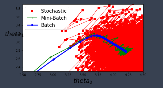
#用小批量梯度下降求解线性回归
theta_path_mgd = []

n_iterations = 50
minibatch_size = 20

np.random.seed(42)
theta = np.random.randn(2,1) #random intialization

for epoch in range(n_iterations):
    shuffled_indices = np.random.permutation(m)
    x_b_shuffled = x_b[shuffled_indices]
    y_shuffled = y[shuffled_indices]
    for i in range(0,m,minibatch_size):
        xi = x_b_shuffled[i:i+minibatch_size]
        yi = y_shuffled[i:i+minibatch_size]
        gradients = 2/minibatch_size * xi.T.dot(xi.dot(theta) - yi)
        eta = 0.1
        theta = theta - eta * gradients
        theta_path_mgd.append(theta)
theta_path_bgd = np.array(theta_path_bgd)
theta_path_sgd = np.array(theta_path_sgd)
theta_path_mgd = np.array(theta_path_mgd)

plt.figure(figsize = (7,4))
plt.plot(theta_path_sgd[:,0],theta_path_sgd[:,1],"r-s",linewidth=1,label="Stochastic")
plt.plot(theta_path_mgd[:,0],theta_path_mgd[:,1],"g-+",linewidth=2,label="Mini-Batch")
plt.plot(theta_path_bgd[:,0],theta_path_bgd[:,1],"b-o",linewidth=3,label="Batch")
plt.legend(loc="upper left",fontsize=16)
plt.xlabel(r"$theta_0$",fontsize=20)
plt.ylabel(r"$theta_1$",fontsize=20,rotation = 0)
plt.axis([2.5,4.5,2.3,3.9])
save_fig("gradients_descent_paths_plot")
plt.show()
参考:https://blog.csdn.net/weixin_36365168/article/details/112484422