python代码:
1.#引入 tensorflow 和 numpy 模块
>>> import tensorflow as tf
>>> import numpy as np
2.#使用numpy模块里的方法生成假数据,总共100个点
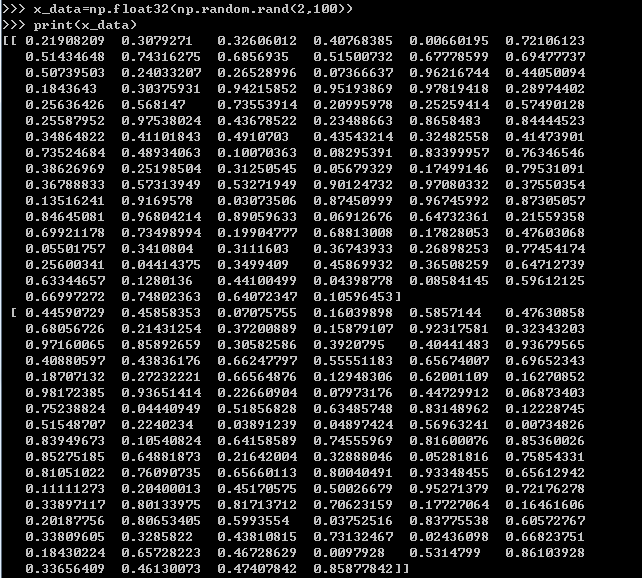
>>> x_data=np.float32(np.random.rand(2,100))
>>> print(x_data)
[[ 0.21908209 0.3079271 0.32606012 0.40768385 0.00660195 0.72106123
0.51434648 0.74316275 0.6856935 0.51500732 0.67778599 0.69477737
0.50739503 0.24033207 0.26528996 0.07366637 0.96216744 0.44050094
0.1843643 0.30375931 0.94215852 0.95193869 0.97819418 0.28974402
0.25636426 0.568147 0.73553914 0.20995978 0.25259414 0.57490128
0.25587952 0.97538024 0.43678522 0.23488663 0.8658483 0.84444523
0.34864822 0.41101843 0.4910703 0.43543214 0.32482558 0.41473901
0.73524684 0.48934063 0.10070363 0.08295391 0.83399957 0.76346546
0.38626969 0.25198504 0.31250545 0.05679329 0.17499146 0.79531091
0.36788833 0.57313949 0.53271949 0.90124732 0.97080332 0.37550354
0.13516241 0.9169578 0.03073506 0.87450999 0.96745992 0.87305057
0.84645081 0.96804214 0.89059633 0.06912676 0.64732361 0.21559358
0.69921178 0.73498994 0.19904777 0.68813008 0.17828053 0.47603068
0.05501757 0.3410804 0.3111603 0.36743933 0.26898253 0.77454174
0.25600341 0.04414375 0.3499409 0.45869932 0.36508259 0.64712739
0.63344657 0.1280136 0.44100499 0.04398778 0.08584145 0.59612125
0.66997272 0.74802363 0.64072347 0.10596453]
[ 0.44590729 0.45858353 0.07075755 0.16039898 0.5857144 0.47630858
0.68056726 0.21431254 0.37200889 0.15879107 0.92317581 0.32343203
0.97160065 0.85892659 0.30582586 0.3920795 0.40441483 0.93679565
0.40880597 0.43836176 0.66247797 0.55551183 0.65674007 0.69652343
0.18707132 0.27232221 0.66564876 0.12948306 0.62001109 0.16270852
0.98172385 0.93651414 0.22660904 0.07973176 0.44729912 0.06873403
0.75238824 0.04440949 0.51856828 0.63485748 0.83148962 0.12228745
0.51548707 0.2240234 0.03891239 0.04897424 0.56963241 0.00734826
0.83949673 0.10540824 0.64158589 0.74555969 0.81600076 0.85360026
0.85275185 0.64881873 0.21642004 0.32888046 0.05281816 0.75854331
0.81051022 0.76090735 0.65660113 0.80040491 0.93348455 0.65612942
0.11111273 0.20400013 0.45170575 0.50026679 0.95271379 0.72176278
0.33897117 0.80133975 0.81713712 0.70623159 0.17727064 0.16461606
0.20187756 0.80653405 0.5993554 0.03752516 0.83775538 0.60572767
0.33809605 0.3285822 0.43810815 0.73132467 0.02436098 0.66823751
0.18430224 0.65728223 0.46728629 0.0097928 0.5314799 0.86103928
0.33656409 0.46130073 0.47407842 0.85877842]]
>>> y_data=np.dot([0.100,0.200],x_data)+0.300
>>> print(y_data)
[ 0.41108967 0.42250942 0.34675752 0.37284818 0.41780308 0.46736784
0.4875481 0.41717878 0.44297113 0.38325894 0.55241376 0.43416414
0.54505963 0.49581853 0.38769417 0.38578254 0.47709971 0.53140922
0.40019762 0.41804828 0.52671145 0.50629624 0.52916743 0.46827909
0.36305069 0.41127914 0.50668367 0.34689259 0.44926163 0.39003183
0.52193272 0.58484085 0.38900033 0.33943502 0.47604465 0.39819133
0.48534247 0.34998374 0.45282069 0.47051471 0.49878048 0.36593139
0.4766221 0.39373874 0.31785284 0.31809024 0.49732644 0.3778162
0.50652632 0.34628015 0.45956772 0.45479127 0.4806993 0.55025114
0.5073392 0.4870777 0.39655596 0.45590082 0.40764396 0.48925902
0.47561828 0.54387725 0.43439373 0.54753198 0.5834429 0.51853094
0.40686763 0.43760424 0.47940078 0.40696603 0.55527512 0.46591191
0.43771541 0.53376694 0.4833322 0.51005933 0.35328218 0.38052628
0.34587727 0.49541485 0.45098711 0.34424896 0.49444933 0.49859971
0.39321955 0.37013081 0.42261572 0.49213487 0.34138045 0.49836024
0.40020511 0.44425781 0.43755776 0.30635734 0.41488012 0.53181998
0.43431009 0.46706251 0.45888803 0.48235214]
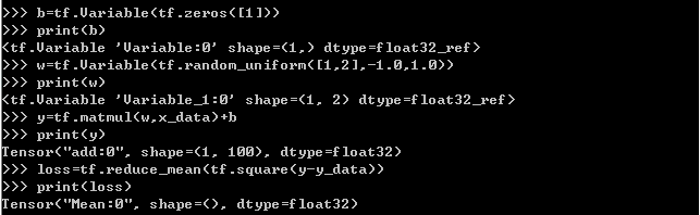
3.#构造一个线性模型
>>> b=tf.Variable(tf.zeros([1]))
>>> print(b)
<tf.Variable 'Variable:0' shape=(1,) dtype=float32_ref>
>>> w=tf.Variable(tf.random_uniform([1,2],-1.0,1.0))
>>> print(w)
<tf.Variable 'Variable_1:0' shape=(1, 2) dtype=float32_ref>
>>> y=tf.matmul(w,x_data)+b
>>> print(y)
Tensor("add:0", shape=(1, 100), dtype=float32)
4.#最小化方差
>>> loss=tf.reduce_mean(tf.square(y-y_data))
>>> print(loss)
Tensor("Mean:0", shape=(), dtype=float32)
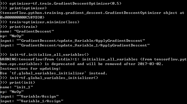
>>> optimizer=tf.train.GradientDescentOptimizer(0.5)
>>> print(optimizer)
<tensorflow.python.training.gradient_descent.GradientDescentOptimizer object at
0x000000000C589D30>
>>> train=optimizer.minimize(loss)
>>> print(train)
name: "GradientDescent"
op: "NoOp"
input: "^GradientDescent/update_Variable/ApplyGradientDescent"
input: "^GradientDescent/update_Variable_1/ApplyGradientDescent"
5.#初始化变量
>>> init=tf.global_variables_initializer()
>>> print(init)
name: "init_1"
op: "NoOp"
input: "^Variable/Assign"
input: "^Variable_1/Assign"
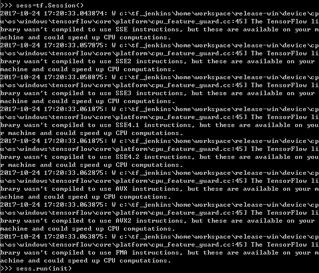
6.#启动图 (graph)
>>> sess=tf.Session()
2017-10-24 17:20:33.043874: W c: f_jenkinshomeworkspace
elease-windevicecp
uoswindows ensorflowcoreplatformcpu_feature_guard.cc:45] The TensorFlow li
brary wasn't compiled to use SSE instructions, but these are available on your m
achine and could speed up CPU computations.
2017-10-24 17:20:33.057875: W c: f_jenkinshomeworkspace
elease-windevicecp
uoswindows ensorflowcoreplatformcpu_feature_guard.cc:45] The TensorFlow li
brary wasn't compiled to use SSE2 instructions, but these are available on your
machine and could speed up CPU computations.
2017-10-24 17:20:33.058875: W c: f_jenkinshomeworkspace
elease-windevicecp
uoswindows ensorflowcoreplatformcpu_feature_guard.cc:45] The TensorFlow li
brary wasn't compiled to use SSE3 instructions, but these are available on your
machine and could speed up CPU computations.
2017-10-24 17:20:33.061875: W c: f_jenkinshomeworkspace
elease-windevicecp
uoswindows ensorflowcoreplatformcpu_feature_guard.cc:45] The TensorFlow li
brary wasn't compiled to use SSE4.1 instructions, but these are available on you
r machine and could speed up CPU computations.
2017-10-24 17:20:33.061875: W c: f_jenkinshomeworkspace
elease-windevicecp
uoswindows ensorflowcoreplatformcpu_feature_guard.cc:45] The TensorFlow li
brary wasn't compiled to use SSE4.2 instructions, but these are available on you
r machine and could speed up CPU computations.
2017-10-24 17:20:33.062875: W c: f_jenkinshomeworkspace
elease-windevicecp
uoswindows ensorflowcoreplatformcpu_feature_guard.cc:45] The TensorFlow li
brary wasn't compiled to use AVX instructions, but these are available on your m
achine and could speed up CPU computations.
2017-10-24 17:20:33.063875: W c: f_jenkinshomeworkspace
elease-windevicecp
uoswindows ensorflowcoreplatformcpu_feature_guard.cc:45] The TensorFlow li
brary wasn't compiled to use AVX2 instructions, but these are available on your
machine and could speed up CPU computations.
2017-10-24 17:20:33.063875: W c: f_jenkinshomeworkspace
elease-windevicecp
uoswindows ensorflowcoreplatformcpu_feature_guard.cc:45] The TensorFlow li
brary wasn't compiled to use FMA instructions, but these are available on your m
achine and could speed up CPU computations.
>>> sess.run(init)
7.#拟合平面结果
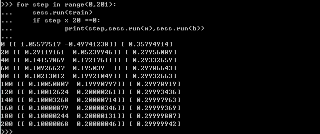
>>> for step in range(0,201):
... sess.run(train)
... if step % 20 ==0:
... print(step,sess.run(w),sess.run(b))
...
0 [[ 1.05577517 -0.49741238]] [ 0.35794914]
20 [[ 0.29119161 0.05239946]] [ 0.27956089]
40 [[ 0.14157869 0.17217611]] [ 0.29332659]
60 [[ 0.10926627 0.195039 ]] [ 0.29786643]
80 [[ 0.10213012 0.19921049]] [ 0.29932663]
100 [[ 0.10050807 0.19990797]] [ 0.29978919]
120 [[ 0.10012624 0.20000261]] [ 0.29993436]
140 [[ 0.10003268 0.20000714]] [ 0.29997963]
160 [[ 0.10000879 0.20000346]] [ 0.29999369]
180 [[ 0.10000244 0.20000131]] [ 0.29999807]
200 [[ 0.10000068 0.20000046]] [ 0.29999942]
预期最佳拟合结果是:w:[[0.100 0.200]],b:[0.300]
结论:随着step的增多,程序实际结果越来越接近预期最佳拟合结果
============================================================
附图: