This is a short introduction to pandas, geared mainly for new users. You can see more complex recipes in the Cookbook.
Customarily, we import as follows:
import numpy as np
import pandas as pd
Object creation
See the Data Structure Intro section.
Creating a Series by passing a list of values, letting pandas create a default integer index:
s = pd.Series([1, 3, 5, np.nan, 6, 8])
s
Out[4]:
0    1.0
1    3.0
2    5.0
3    NaN
4    6.0
5    8.0
dtype: float64
Creating a DataFrame by passing a NumPy array, with a datetime index and labeled columns:
dates = pd.date_range("20130101", periods=6)
dates
Out[6]:
DatetimeIndex(['2013-01-01', '2013-01-02', '2013-01-03', '2013-01-04',
               '2013-01-05', '2013-01-06'],
              dtype='datetime64[ns]', freq='D')
df = pd.DataFrame(np.random.randn(6, 4), index=dates, columns=list("ABCD"))
df
Out[8]:
                   A         B         C         D
2013-01-01  0.469112 -0.282863 -1.509059 -1.135632
2013-01-02  1.212112 -0.173215  0.119209 -1.044236
2013-01-03 -0.861849 -2.104569 -0.494929  1.071804
2013-01-04  0.721555 -0.706771 -1.039575  0.271860
2013-01-05 -0.424972  0.567020  0.276232 -1.087401
2013-01-06 -0.673690  0.113648 -1.478427  0.524988
Creating a DataFrame by passing a dict of objects that can be converted to series-like.
df2 = pd.DataFrame(
{
"A": 1.0,
"B": pd.Timestamp("20130102"),
"C": pd.Series(1, index=list(range(4)), dtype="float32"),
"D": np.array([3] * 4, dtype="int32"),
"E": pd.Categorical(["test", "train", "test", "train"]),
"F": "foo",
}
)
df2
Out[10]:
     A          B    C  D      E    F
0  1.0 2013-01-02  1.0  3   test  foo
1  1.0 2013-01-02  1.0  3  train  foo
2  1.0 2013-01-02  1.0  3   test  foo
3  1.0 2013-01-02  1.0  3  train  foo
The columns of the resulting DataFrame have different dtypes.
df2.dtypes
Out[11]:
A           float64
B    datetime64[ns]
C           float32
D             int32
E          category
F            object
dtype: object
If you’re using IPython, tab completion for column names (as well as public attributes) is automatically enabled. Here’s a subset of the attributes that will be completed:
df2.<TAB>  # noqa: E225, E999
df2.A                  df2.bool
df2.abs                df2.boxplot
df2.add                df2.C
df2.add_prefix         df2.clip
df2.add_suffix         df2.columns
df2.align              df2.copy
df2.all                df2.count
df2.any                df2.combine
df2.append             df2.D
df2.apply              df2.describe
df2.applymap           df2.diff
df2.B                  df2.duplicated
As you can see, the columns A, B, C, and D are automatically tab completed. E and F are there as well; the rest of the attributes have been truncated for brevity.
Viewing data
See the Basics section.
Here is how to view the top and bottom rows of the frame:
df.head()
Out[13]:
                   A         B         C         D
2013-01-01  0.469112 -0.282863 -1.509059 -1.135632
2013-01-02  1.212112 -0.173215  0.119209 -1.044236
2013-01-03 -0.861849 -2.104569 -0.494929  1.071804
2013-01-04  0.721555 -0.706771 -1.039575  0.271860
2013-01-05 -0.424972  0.567020  0.276232 -1.087401
df.tail(3)
Out[14]:
                   A         B         C         D
2013-01-04  0.721555 -0.706771 -1.039575  0.271860
2013-01-05 -0.424972  0.567020  0.276232 -1.087401
2013-01-06 -0.673690  0.113648 -1.478427  0.524988
Display the index, columns:
df.index
Out[15]:
DatetimeIndex(['2013-01-01', '2013-01-02', '2013-01-03', '2013-01-04',
               '2013-01-05', '2013-01-06'],
              dtype='datetime64[ns]', freq='D')
df.columns
Out[16]: Index(['A', 'B', 'C', 'D'], dtype='object')
DataFrame.to_numpy() gives a NumPy representation of the underlying data. Note that this can be an expensive operation when your DataFrame has columns with different data types, which comes down to a fundamental difference between pandas and NumPy: NumPy arrays have one dtype for the entire array, while pandas DataFrames have one dtype per column. When you call DataFrame.to_numpy(), pandas will find the NumPy dtype that can hold all of the dtypes in the DataFrame. This may end up being object, which requires casting every value to a Python object.
For df, our DataFrame of all floating-point values, DataFrame.to_numpy() is fast and doesn’t require copying data.
df.to_numpy()
Out[17]:
array([[ 0.4691, -0.2829, -1.5091, -1.1356],
       [ 1.2121, -0.1732,  0.1192, -1.0442],
       [-0.8618, -2.1046, -0.4949,  1.0718],
       [ 0.7216, -0.7068, -1.0396,  0.2719],
       [-0.425 ,  0.567 ,  0.2762, -1.0874],
       [-0.6737,  0.1136, -1.4784,  0.525 ]])
For df2, the DataFrame with multiple dtypes, DataFrame.to_numpy() is relatively expensive.
df2.to_numpy()
Out[18]:
array([[1.0, Timestamp('2013-01-02 00:00:00'), 1.0, 3, 'test', 'foo'],
       [1.0, Timestamp('2013-01-02 00:00:00'), 1.0, 3, 'train', 'foo'],
       [1.0, Timestamp('2013-01-02 00:00:00'), 1.0, 3, 'test', 'foo'],
       [1.0, Timestamp('2013-01-02 00:00:00'), 1.0, 3, 'train', 'foo']],
      dtype=object)
Note
DataFrame.to_numpy() does not include the index or column labels in the output.
describe() shows a quick statistic summary of your data:
df.describe()
Out[19]:
              A         B         C         D
count  6.000000  6.000000  6.000000  6.000000
mean   0.073711 -0.431125 -0.687758 -0.233103
std    0.843157  0.922818  0.779887  0.973118
min   -0.861849 -2.104569 -1.509059 -1.135632
25%   -0.611510 -0.600794 -1.368714 -1.076610
50%    0.022070 -0.228039 -0.767252 -0.386188
75%    0.658444  0.041933 -0.034326  0.461706
max    1.212112  0.567020  0.276232  1.071804
Transposing your data:
df.T
Out[20]:
   2013-01-01  2013-01-02  2013-01-03  2013-01-04  2013-01-05  2013-01-06
A    0.469112    1.212112   -0.861849    0.721555   -0.424972   -0.673690
B   -0.282863   -0.173215   -2.104569   -0.706771    0.567020    0.113648
C   -1.509059    0.119209   -0.494929   -1.039575    0.276232   -1.478427
D   -1.135632   -1.044236    1.071804    0.271860   -1.087401    0.524988
Sorting by an axis:
df.sort_index(axis=1, ascending=False)
Out[21]:
                   D         C         B         A
2013-01-01 -1.135632 -1.509059 -0.282863  0.469112
2013-01-02 -1.044236  0.119209 -0.173215  1.212112
2013-01-03  1.071804 -0.494929 -2.104569 -0.861849
2013-01-04  0.271860 -1.039575 -0.706771  0.721555
2013-01-05 -1.087401  0.276232  0.567020 -0.424972
2013-01-06  0.524988 -1.478427  0.113648 -0.673690
Sorting by values:
df.sort_values(by="B")
Out[22]:
                   A         B         C         D
2013-01-03 -0.861849 -2.104569 -0.494929  1.071804
2013-01-04  0.721555 -0.706771 -1.039575  0.271860
2013-01-01  0.469112 -0.282863 -1.509059 -1.135632
2013-01-02  1.212112 -0.173215  0.119209 -1.044236
2013-01-06 -0.673690  0.113648 -1.478427  0.524988
2013-01-05 -0.424972  0.567020  0.276232 -1.087401
Selection
Note
While standard Python / NumPy expressions for selecting and setting are intuitive and come in handy for interactive work, for production code, we recommend the optimized pandas data access methods, .at, .iat, .loc and .iloc.
See the indexing documentation Indexing and Selecting Data and MultiIndex / Advanced Indexing.
Getting
Selecting a single column, which yields a Series, equivalent to df.A:
df["A"]
Out[23]:
2013-01-01    0.469112
2013-01-02    1.212112
2013-01-03   -0.861849
2013-01-04    0.721555
2013-01-05   -0.424972
2013-01-06   -0.673690
Freq: D, Name: A, dtype: float64
Selecting via [], which slices the rows.
df[0:3]
Out[24]:
                   A         B         C         D
2013-01-01  0.469112 -0.282863 -1.509059 -1.135632
2013-01-02  1.212112 -0.173215  0.119209 -1.044236
2013-01-03 -0.861849 -2.104569 -0.494929  1.071804
df["20130102":"20130104"]
Out[25]:
                   A         B         C         D
2013-01-02  1.212112 -0.173215  0.119209 -1.044236
2013-01-03 -0.861849 -2.104569 -0.494929  1.071804
2013-01-04  0.721555 -0.706771 -1.039575  0.271860
Selection by label
See more in Selection by Label.
For getting a cross section using a label:
df.loc[dates[0]]
Out[26]:
A    0.469112
B   -0.282863
C   -1.509059
D   -1.135632
Name: 2013-01-01 00:00:00, dtype: float64
Selecting on a multi-axis by label:
df.loc[:, ["A", "B"]]
Out[27]:
                   A         B
2013-01-01  0.469112 -0.282863
2013-01-02  1.212112 -0.173215
2013-01-03 -0.861849 -2.104569
2013-01-04  0.721555 -0.706771
2013-01-05 -0.424972  0.567020
2013-01-06 -0.673690  0.113648
Showing label slicing, both endpoints are included:
df.loc["20130102":"20130104", ["A", "B"]]
Out[28]:
                   A         B
2013-01-02  1.212112 -0.173215
2013-01-03 -0.861849 -2.104569
2013-01-04  0.721555 -0.706771
Reduction in the dimensions of the returned object:
df.loc["20130102", ["A", "B"]]
Out[29]:
A    1.212112
B   -0.173215
Name: 2013-01-02 00:00:00, dtype: float64
For getting a scalar value:
df.loc[dates[0], "A"]
Out[30]: 0.4691122999071863
For getting fast access to a scalar (equivalent to the prior method):
df.at[dates[0], "A"]
Out[31]: 0.4691122999071863
Selection by position
See more in Selection by Position.
Select via the position of the passed integers:
df.iloc[3]
Out[32]:
A    0.721555
B   -0.706771
C   -1.039575
D    0.271860
Name: 2013-01-04 00:00:00, dtype: float64
By integer slices, acting similar to NumPy/Python:
df.iloc[3:5, 0:2]
Out[33]:
                   A         B
2013-01-04  0.721555 -0.706771
2013-01-05 -0.424972  0.567020
By lists of integer position locations, similar to the NumPy/Python style:
df.iloc[[1, 2, 4], [0, 2]]
Out[34]:
                   A         C
2013-01-02  1.212112  0.119209
2013-01-03 -0.861849 -0.494929
2013-01-05 -0.424972  0.276232
For slicing rows explicitly:
df.iloc[1:3, :]
Out[35]:
                   A         B         C         D
2013-01-02  1.212112 -0.173215  0.119209 -1.044236
2013-01-03 -0.861849 -2.104569 -0.494929  1.071804
For slicing columns explicitly:
df.iloc[:, 1:3]
Out[36]:
                   B         C
2013-01-01 -0.282863 -1.509059
2013-01-02 -0.173215  0.119209
2013-01-03 -2.104569 -0.494929
2013-01-04 -0.706771 -1.039575
2013-01-05  0.567020  0.276232
2013-01-06  0.113648 -1.478427
For getting a value explicitly:
df.iloc[1, 1]
Out[37]: -0.17321464905330858
For getting fast access to a scalar (equivalent to the prior method):
df.iat[1, 1]
Out[38]: -0.17321464905330858
Boolean indexing
Using a single column’s values to select data.
df[df["A"] > 0]
Out[39]:
                   A         B         C         D
2013-01-01  0.469112 -0.282863 -1.509059 -1.135632
2013-01-02  1.212112 -0.173215  0.119209 -1.044236
2013-01-04  0.721555 -0.706771 -1.039575  0.271860
Selecting values from a DataFrame where a boolean condition is met.
df[df > 0]
Out[40]:
                   A         B         C         D
2013-01-01  0.469112       NaN       NaN       NaN
2013-01-02  1.212112       NaN  0.119209       NaN
2013-01-03       NaN       NaN       NaN  1.071804
2013-01-04  0.721555       NaN       NaN  0.271860
2013-01-05       NaN  0.567020  0.276232       NaN
2013-01-06       NaN  0.113648       NaN  0.524988
Using the isin() method for filtering:
df2 = df.copy()
df2["E"] = ["one", "one", "two", "three", "four", "three"]
df2
Out[43]:
                   A         B         C         D      E
2013-01-01  0.469112 -0.282863 -1.509059 -1.135632    one
2013-01-02  1.212112 -0.173215  0.119209 -1.044236    one
2013-01-03 -0.861849 -2.104569 -0.494929  1.071804    two
2013-01-04  0.721555 -0.706771 -1.039575  0.271860  three
2013-01-05 -0.424972  0.567020  0.276232 -1.087401   four
2013-01-06 -0.673690  0.113648 -1.478427  0.524988  three
df2[df2["E"].isin(["two", "four"])]
Out[44]:
                   A         B         C         D     E
2013-01-03 -0.861849 -2.104569 -0.494929  1.071804   two
2013-01-05 -0.424972  0.567020  0.276232 -1.087401  four
Setting
Setting a new column automatically aligns the data by the indexes.
s1 = pd.Series([1, 2, 3, 4, 5, 6], index=pd.date_range("20130102", periods=6))
s1
Out[46]:
2013-01-02    1
2013-01-03    2
2013-01-04    3
2013-01-05    4
2013-01-06    5
2013-01-07    6
Freq: D, dtype: int64
df["F"] = s1
Setting values by label:
df.at[dates[0], "A"] = 0
Setting values by position:
df.iat[0, 1] = 0
Setting by assigning with a NumPy array:
df.loc[:, "D"] = np.array([5] * len(df))
The result of the prior setting operations.
df
Out[51]:
                   A         B         C  D    F
2013-01-01  0.000000  0.000000 -1.509059  5  NaN
2013-01-02  1.212112 -0.173215  0.119209  5  1.0
2013-01-03 -0.861849 -2.104569 -0.494929  5  2.0
2013-01-04  0.721555 -0.706771 -1.039575  5  3.0
2013-01-05 -0.424972  0.567020  0.276232  5  4.0
2013-01-06 -0.673690  0.113648 -1.478427  5  5.0
A where operation with setting.
df2 = df.copy()
df2[df2 > 0] = -df2
df2
Out[54]:
                   A         B         C  D    F
2013-01-01  0.000000  0.000000 -1.509059 -5  NaN
2013-01-02 -1.212112 -0.173215 -0.119209 -5 -1.0
2013-01-03 -0.861849 -2.104569 -0.494929 -5 -2.0
2013-01-04 -0.721555 -0.706771 -1.039575 -5 -3.0
2013-01-05 -0.424972 -0.567020 -0.276232 -5 -4.0
2013-01-06 -0.673690 -0.113648 -1.478427 -5 -5.0
Missing data
pandas primarily uses the value np.nan to represent missing data. It is by default not included in computations. See the Missing Data section.
Reindexing allows you to change/add/delete the index on a specified axis. This returns a copy of the data.
df1 = df.reindex(index=dates[0:4], columns=list(df.columns) + ["E"])
df1.loc[dates[0] : dates[1], "E"] = 1
df1
Out[57]:
                   A         B         C  D    F    E
2013-01-01  0.000000  0.000000 -1.509059  5  NaN  1.0
2013-01-02  1.212112 -0.173215  0.119209  5  1.0  1.0
2013-01-03 -0.861849 -2.104569 -0.494929  5  2.0  NaN
2013-01-04  0.721555 -0.706771 -1.039575  5  3.0  NaN
To drop any rows that have missing data.
df1.dropna(how="any")
Out[58]:
                   A         B         C  D    F    E
2013-01-02  1.212112 -0.173215  0.119209  5  1.0  1.0
Filling missing data.
df1.fillna(value=5)
Out[59]:
                   A         B         C  D    F    E
2013-01-01  0.000000  0.000000 -1.509059  5  5.0  1.0
2013-01-02  1.212112 -0.173215  0.119209  5  1.0  1.0
2013-01-03 -0.861849 -2.104569 -0.494929  5  2.0  5.0
2013-01-04  0.721555 -0.706771 -1.039575  5  3.0  5.0
To get the boolean mask where values are nan.
pd.isna(df1)
Out[60]:
                A      B      C      D      F      E
2013-01-01  False  False  False  False   True  False
2013-01-02  False  False  False  False  False  False
2013-01-03  False  False  False  False  False   True
2013-01-04  False  False  False  False  False   True
Operations
See the Basic section on Binary Ops.
Stats
Operations in general exclude missing data.
Performing a descriptive statistic:
df.mean()
Out[61]:
A   -0.004474
B   -0.383981
C   -0.687758
D    5.000000
F    3.000000
dtype: float64
Same operation on the other axis:
df.mean(1)
Out[62]:
2013-01-01    0.872735
2013-01-02    1.431621
2013-01-03    0.707731
2013-01-04    1.395042
2013-01-05    1.883656
2013-01-06    1.592306
Freq: D, dtype: float64
Operating with objects that have different dimensionality and need alignment. In addition, pandas automatically broadcasts along the specified dimension.
s = pd.Series([1, 3, 5, np.nan, 6, 8], index=dates).shift(2)
s
Out[64]:
2013-01-01    NaN
2013-01-02    NaN
2013-01-03    1.0
2013-01-04    3.0
2013-01-05    5.0
2013-01-06    NaN
Freq: D, dtype: float64
df.sub(s, axis="index")
Out[65]:
                   A         B         C    D    F
2013-01-01       NaN       NaN       NaN  NaN  NaN
2013-01-02       NaN       NaN       NaN  NaN  NaN
2013-01-03 -1.861849 -3.104569 -1.494929  4.0  1.0
2013-01-04 -2.278445 -3.706771 -4.039575  2.0  0.0
2013-01-05 -5.424972 -4.432980 -4.723768  0.0 -1.0
2013-01-06       NaN       NaN       NaN  NaN  NaN
Apply
Applying functions to the data:
df.apply(np.cumsum)
Out[66]:
                   A         B         C   D     F
2013-01-01  0.000000  0.000000 -1.509059   5   NaN
2013-01-02  1.212112 -0.173215 -1.389850  10   1.0
2013-01-03  0.350263 -2.277784 -1.884779  15   3.0
2013-01-04  1.071818 -2.984555 -2.924354  20   6.0
2013-01-05  0.646846 -2.417535 -2.648122  25  10.0
2013-01-06 -0.026844 -2.303886 -4.126549  30  15.0
df.apply(lambda x: x.max() - x.min())
Out[67]:
A    2.073961
B    2.671590
C    1.785291
D    0.000000
F    4.000000
dtype: float64
Histogramming
See more at Histogramming and Discretization.
s = pd.Series(np.random.randint(0, 7, size=10))
s
Out[69]:
0    4
1    2
2    1
3    2
4    6
5    4
6    4
7    6
8    4
9    4
dtype: int64
s.value_counts()
Out[70]:
4    5
2    2
6    2
1    1
dtype: int64
String Methods
Series is equipped with a set of string processing methods in the str attribute that make it easy to operate on each element of the array, as in the code snippet below. Note that pattern-matching in str generally uses regular expressions by default (and in some cases always uses them). See more at Vectorized String Methods.
s = pd.Series(["A", "B", "C", "Aaba", "Baca", np.nan, "CABA", "dog", "cat"])
s.str.lower()
Out[72]:
0       a
1       b
2       c
3    aaba
4    baca
5     NaN
6    caba
7     dog
8     cat
dtype: object
Merge
Concat
pandas provides various facilities for easily combining together Series and DataFrame objects with various kinds of set logic for the indexes and relational algebra functionality in the case of join / merge-type operations.
See the Merging section.
Concatenating pandas objects together with concat():
df = pd.DataFrame(np.random.randn(10, 4))
df
Out[74]:
          0         1         2         3
0 -0.548702  1.467327 -1.015962 -0.483075
1  1.637550 -1.217659 -0.291519 -1.745505
2 -0.263952  0.991460 -0.919069  0.266046
3 -0.709661  1.669052  1.037882 -1.705775
4 -0.919854 -0.042379  1.247642 -0.009920
5  0.290213  0.495767  0.362949  1.548106
6 -1.131345 -0.089329  0.337863 -0.945867
7 -0.932132  1.956030  0.017587 -0.016692
8 -0.575247  0.254161 -1.143704  0.215897
9  1.193555 -0.077118 -0.408530 -0.862495

# break it into pieces
pieces = [df[:3], df[3:7], df[7:]]
pd.concat(pieces)
Out[76]:
          0         1         2         3
0 -0.548702  1.467327 -1.015962 -0.483075
1  1.637550 -1.217659 -0.291519 -1.745505
2 -0.263952  0.991460 -0.919069  0.266046
3 -0.709661  1.669052  1.037882 -1.705775
4 -0.919854 -0.042379  1.247642 -0.009920
5  0.290213  0.495767  0.362949  1.548106
6 -1.131345 -0.089329  0.337863 -0.945867
7 -0.932132  1.956030  0.017587 -0.016692
8 -0.575247  0.254161 -1.143704  0.215897
9  1.193555 -0.077118 -0.408530 -0.862495
Note
Adding a column to a DataFrame is relatively fast. However, adding a row requires a copy, and may be expensive. We recommend passing a pre-built list of records to the DataFrame constructor instead of building a DataFrame by iteratively appending records to it. See Appending to dataframe for more.
Join
SQL style merges. See the Database style joining section.
left = pd.DataFrame({"key": ["foo", "foo"], "lval": [1, 2]})
right = pd.DataFrame({"key": ["foo", "foo"], "rval": [4, 5]})
left
Out[79]:
   key  lval
0  foo     1
1  foo     2
right
Out[80]:
   key  rval
0  foo     4
1  foo     5
pd.merge(left, right, on="key")
Out[81]:
   key  lval  rval
0  foo     1     4
1  foo     1     5
2  foo     2     4
3  foo     2     5
Another example that can be given is:
left = pd.DataFrame({"key": ["foo", "bar"], "lval": [1, 2]})
right = pd.DataFrame({"key": ["foo", "bar"], "rval": [4, 5]})
left
Out[84]:
   key  lval
0  foo     1
1  bar     2
right
Out[85]:
   key  rval
0  foo     4
1  bar     5
pd.merge(left, right, on="key")
Out[86]:
   key  lval  rval
0  foo     1     4
1  bar     2     5
Grouping
By “group by” we are referring to a process involving one or more of the following steps:
Splitting the data into groups based on some criteria
Applying a function to each group independently
Combining the results into a data structure
See the Grouping section.
df = pd.DataFrame(
{
"A": ["foo", "bar", "foo", "bar", "foo", "bar", "foo", "foo"],
"B": ["one", "one", "two", "three", "two", "two", "one", "three"],
"C": np.random.randn(8),
"D": np.random.randn(8),
}
)
df
Out[88]:
     A      B         C         D
0  foo    one  1.346061 -1.577585
1  bar    one  1.511763  0.396823
2  foo    two  1.627081 -0.105381
3  bar  three -0.990582 -0.532532
4  foo    two -0.441652  1.453749
5  bar    two  1.211526  1.208843
6  foo    one  0.268520 -0.080952
7  foo  three  0.024580 -0.264610
Grouping and then applying the sum() function to the resulting groups.
df.groupby("A").sum()
Out[89]:
            C         D
A
bar  1.732707  1.073134
foo  2.824590 -0.574779
Grouping by multiple columns forms a hierarchical index, and again we can apply the sum() function.
df.groupby(["A", "B"]).sum()
Out[90]:
                  C         D
A   B
bar one    1.511763  0.396823
    three -0.990582 -0.532532
    two    1.211526  1.208843
foo one    1.614581 -1.658537
    three  0.024580 -0.264610
    two    1.185429  1.348368
Reshaping
See the sections on Hierarchical Indexing and Reshaping.
Stack
tuples = list(
zip(
*[
["bar", "bar", "baz", "baz", "foo", "foo", "qux", "qux"],
["one", "two", "one", "two", "one", "two", "one", "two"],
]
)
)
index = pd.MultiIndex.from_tuples(tuples, names=["first", "second"])
df = pd.DataFrame(np.random.randn(8, 2), index=index, columns=["A", "B"])
df2 = df[:4]
df2
Out[95]:
                     A         B
first second
bar   one    -0.727965 -0.589346
      two     0.339969 -0.693205
baz   one    -0.339355  0.593616
      two     0.884345  1.591431
The stack() method “compresses” a level in the DataFrame’s columns.
stacked = df2.stack()
stacked
Out[97]:
first  second
bar    one     A   -0.727965
               B   -0.589346
       two     A    0.339969
               B   -0.693205
baz    one     A   -0.339355
               B    0.593616
       two     A    0.884345
               B    1.591431
dtype: float64
With a “stacked” DataFrame or Series (having a MultiIndex as the index), the inverse operation of stack() is unstack(), which by default unstacks the last level:
stacked.unstack()
Out[98]:
                     A         B
first second
bar   one    -0.727965 -0.589346
      two     0.339969 -0.693205
baz   one    -0.339355  0.593616
      two     0.884345  1.591431
stacked.unstack(1)
Out[99]:
second        one       two
first
bar   A -0.727965  0.339969
      B -0.589346 -0.693205
baz   A -0.339355  0.884345
      B  0.593616  1.591431
stacked.unstack(0)
Out[100]:
first          bar       baz
second
one    A -0.727965 -0.339355
       B -0.589346  0.593616
two    A  0.339969  0.884345
       B -0.693205  1.591431
Pivot tables
See the section on Pivot Tables.
df = pd.DataFrame(
{
"A": ["one", "one", "two", "three"] * 3,
"B": ["A", "B", "C"] * 4,
"C": ["foo", "foo", "foo", "bar", "bar", "bar"] * 2,
"D": np.random.randn(12),
"E": np.random.randn(12),
}
)
df
Out[102]:
        A  B    C         D         E
0     one  A  foo -1.202872  0.047609
1     one  B  foo -1.814470 -0.136473
2     two  C  foo  1.018601 -0.561757
3   three  A  bar -0.595447 -1.623033
4     one  B  bar  1.395433  0.029399
5     one  C  bar -0.392670 -0.542108
6     two  A  foo  0.007207  0.282696
7   three  B  foo  1.928123 -0.087302
8     one  C  foo -0.055224 -1.575170
9     one  A  bar  2.395985  1.771208
10    two  B  bar  1.552825  0.816482
11  three  C  bar  0.166599  1.100230
We can produce pivot tables from this data very easily:
pd.pivot_table(df, values="D", index=["A", "B"], columns=["C"])
Out[103]:
C             bar       foo
A     B
one   A  2.395985 -1.202872
      B  1.395433 -1.814470
      C -0.392670 -0.055224
three A -0.595447       NaN
      B       NaN  1.928123
      C  0.166599       NaN
two   A       NaN  0.007207
      B  1.552825       NaN
      C       NaN  1.018601
Time series
pandas has simple, powerful, and efficient functionality for performing resampling operations during frequency conversion (e.g., converting secondly data into 5-minutely data). This is extremely common in, but not limited to, financial applications. See the Time Series section.
rng = pd.date_range("1/1/2012", periods=100, freq="S")
ts = pd.Series(np.random.randint(0, 500, len(rng)), index=rng)
ts.resample("5Min").sum()
Out[106]:
2012-01-01    24182
Freq: 5T, dtype: int64
Time zone representation:
rng = pd.date_range("3/6/2012 00:00", periods=5, freq="D")
ts = pd.Series(np.random.randn(len(rng)), rng)
ts
Out[109]:
2012-03-06    1.857704
2012-03-07   -1.193545
2012-03-08    0.677510
2012-03-09   -0.153931
2012-03-10    0.520091
Freq: D, dtype: float64
ts_utc = ts.tz_localize("UTC")
ts_utc
Out[111]:
2012-03-06 00:00:00+00:00    1.857704
2012-03-07 00:00:00+00:00   -1.193545
2012-03-08 00:00:00+00:00    0.677510
2012-03-09 00:00:00+00:00   -0.153931
2012-03-10 00:00:00+00:00    0.520091
Freq: D, dtype: float64
Converting to another time zone:
ts_utc.tz_convert("US/Eastern")
Out[112]:
2012-03-05 19:00:00-05:00    1.857704
2012-03-06 19:00:00-05:00   -1.193545
2012-03-07 19:00:00-05:00    0.677510
2012-03-08 19:00:00-05:00   -0.153931
2012-03-09 19:00:00-05:00    0.520091
Freq: D, dtype: float64
Converting between time span representations:
rng = pd.date_range("1/1/2012", periods=5, freq="M")
ts = pd.Series(np.random.randn(len(rng)), index=rng)
ts
Out[115]:
2012-01-31   -1.475051
2012-02-29    0.722570
2012-03-31   -0.322646
2012-04-30   -1.601631
2012-05-31    0.778033
Freq: M, dtype: float64
ps = ts.to_period()
ps
Out[117]:
2012-01   -1.475051
2012-02    0.722570
2012-03   -0.322646
2012-04   -1.601631
2012-05    0.778033
Freq: M, dtype: float64
ps.to_timestamp()
Out[118]:
2012-01-01   -1.475051
2012-02-01    0.722570
2012-03-01   -0.322646
2012-04-01   -1.601631
2012-05-01    0.778033
Freq: MS, dtype: float64
Converting between period and timestamp enables some convenient arithmetic functions to be used. In the following example, we convert a quarterly frequency with year ending in November to 9am of the end of the month following the quarter end:
prng = pd.period_range("1990Q1", "2000Q4", freq="Q-NOV")
ts = pd.Series(np.random.randn(len(prng)), prng)
ts.index = (prng.asfreq("M", "e") + 1).asfreq("H", "s") + 9
ts.head()
Out[122]:
1990-03-01 09:00   -0.289342
1990-06-01 09:00    0.233141
1990-09-01 09:00   -0.223540
1990-12-01 09:00    0.542054
1991-03-01 09:00   -0.688585
Freq: H, dtype: float64
Categoricals
pandas can include categorical data in a DataFrame. For full docs, see the categorical introduction and the API documentation.
df = pd.DataFrame(
{"id": [1, 2, 3, 4, 5, 6], "raw_grade": ["a", "b", "b", "a", "a", "e"]}
)
Convert the raw grades to a categorical data type.
df["grade"] = df["raw_grade"].astype("category")
df["grade"]
Out[125]:
0    a
1    b
2    b
3    a
4    a
5    e
Name: grade, dtype: category
Categories (3, object): ['a', 'b', 'e']
Rename the categories to more meaningful names (assigning to Series.cat.categories() is in place!).
df["grade"].cat.categories = ["very good", "good", "very bad"]
Reorder the categories and simultaneously add the missing categories (methods under Series.cat() return a new Series by default).
df["grade"] = df["grade"].cat.set_categories(
["very bad", "bad", "medium", "good", "very good"]
)
df["grade"]
Out[128]:
0    very good
1         good
2         good
3    very good
4    very good
5     very bad
Name: grade, dtype: category
Categories (5, object): ['very bad', 'bad', 'medium', 'good', 'very good']
Sorting is per order in the categories, not lexical order.
df.sort_values(by="grade")
Out[129]:
   id raw_grade      grade
5   6         e   very bad
1   2         b       good
2   3         b       good
0   1         a  very good
3   4         a  very good
4   5         a  very good
Grouping by a categorical column also shows empty categories.
df.groupby("grade").size()
Out[130]:
grade
very bad     1
bad          0
medium       0
good         2
very good    3
dtype: int64
Plotting
See the Plotting docs.
We use the standard convention for referencing the matplotlib API:
import matplotlib.pyplot as plt
plt.close("all")
The close() method is used to close a figure window.
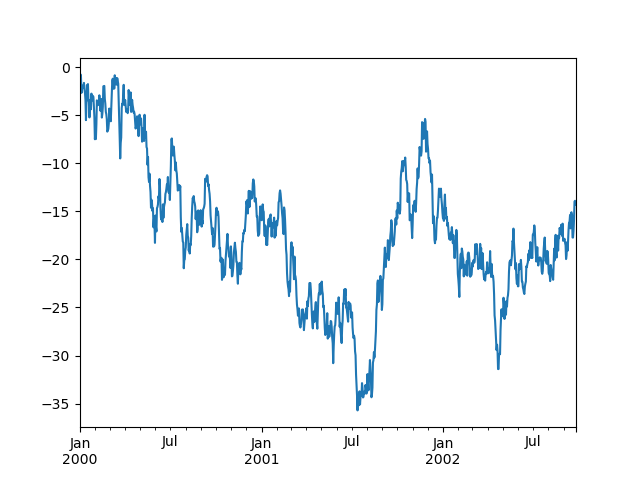
ts = pd.Series(np.random.randn(1000), index=pd.date_range("1/1/2000", periods=1000))
ts = ts.cumsum()
ts.plot();
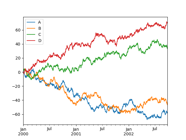
On a DataFrame, the plot() method is a convenience to plot all of the columns with labels:
df = pd.DataFrame(
np.random.randn(1000, 4), index=ts.index, columns=["A", "B", "C", "D"]
)
df = df.cumsum()
plt.figure();
df.plot();
plt.legend(loc='best');
Getting data in/out
CSV
Writing to a csv file.
df.to_csv("foo.csv")
Reading from a csv file.
pd.read_csv("foo.csv")
Out[142]:
     Unnamed: 0          A          B          C          D
0    2000-01-01   0.350262   0.843315   1.798556   0.782234
1    2000-01-02  -0.586873   0.034907   1.923792  -0.562651
2    2000-01-03  -1.245477  -0.963406   2.269575  -1.612566
3    2000-01-04  -0.252830  -0.498066   3.176886  -1.275581
4    2000-01-05  -1.044057   0.118042   2.768571   0.386039
..          ...        ...        ...        ...        ...
995  2002-09-22 -48.017654  31.474551  69.146374 -47.541670
996  2002-09-23 -47.207912  32.627390  68.505254 -48.828331
997  2002-09-24 -48.907133  31.990402  67.310924 -49.391051
998  2002-09-25 -50.146062  33.716770  67.717434 -49.037577
999  2002-09-26 -49.724318  33.479952  68.108014 -48.822030

[1000 rows x 5 columns]
HDF5
Reading and writing to HDFStores.
Writing to a HDF5 Store.
df.to_hdf("foo.h5", "df")
Reading from a HDF5 Store.
pd.read_hdf("foo.h5", "df")
Out[144]:
                    A          B          C          D
2000-01-01   0.350262   0.843315   1.798556   0.782234
2000-01-02  -0.586873   0.034907   1.923792  -0.562651
2000-01-03  -1.245477  -0.963406   2.269575  -1.612566
2000-01-04  -0.252830  -0.498066   3.176886  -1.275581
2000-01-05  -1.044057   0.118042   2.768571   0.386039
...               ...        ...        ...        ...
2002-09-22 -48.017654  31.474551  69.146374 -47.541670
2002-09-23 -47.207912  32.627390  68.505254 -48.828331
2002-09-24 -48.907133  31.990402  67.310924 -49.391051
2002-09-25 -50.146062  33.716770  67.717434 -49.037577
2002-09-26 -49.724318  33.479952  68.108014 -48.822030

[1000 rows x 4 columns]
Excel
Reading and writing to MS Excel.
Writing to an excel file.
df.to_excel("foo.xlsx", sheet_name="Sheet1")
Reading from an excel file.
pd.read_excel("foo.xlsx", "Sheet1", index_col=None, na_values=["NA"])
Out[146]:
    Unnamed: 0          A          B          C          D
0   2000-01-01   0.350262   0.843315   1.798556   0.782234
1   2000-01-02  -0.586873   0.034907   1.923792  -0.562651
2   2000-01-03  -1.245477  -0.963406   2.269575  -1.612566
3   2000-01-04  -0.252830  -0.498066   3.176886  -1.275581
4   2000-01-05  -1.044057   0.118042   2.768571   0.386039
..         ...        ...        ...        ...        ...
995 2002-09-22 -48.017654  31.474551  69.146374 -47.541670
996 2002-09-23 -47.207912  32.627390  68.505254 -48.828331
997 2002-09-24 -48.907133  31.990402  67.310924 -49.391051
998 2002-09-25 -50.146062  33.716770  67.717434 -49.037577
999 2002-09-26 -49.724318  33.479952  68.108014 -48.822030

[1000 rows x 5 columns]
Gotchas
If you are attempting to perform an operation you might see an exception like:
if pd.Series([False, True, False]):
    print("I was true")
Traceback
    ...
ValueError: The truth value of an array is ambiguous. Use a.empty, a.any() or a.all().
See Comparisons for an explanation and what to do.
See Gotchas as well.