Anomaly Detection

       数据集中的异常数据通常被成为异常点、离群点或孤立点等，典型特征是这些数据的特征或规则与大多数数据不一致，呈现出“异常”的特点，而检测这些数据的方法被称为异常检测。

　　异常数据根据原始数据集的不同可以分为离群点检测和新奇检测：

• 离群点检测(Outlier Detection)

　　大多数情况我们定义的异常数据都属于离群点检测，对这些数据训练完之后再在新的数据集中寻找异常点。

• 新奇检测(Novelty Detection)

　　所谓新奇检测是识别新的或未知数据模式和规律的检测方法，这些规律和只是在已有机器学习系统的训练集中没有被发掘出来。新奇检测的前提是已知训练数据集是“纯净”的，未被真正的“噪音”数据或真实的“离群点”污染，然后针对这些数据训练完成之后再对新的数据做训练以寻找新奇数据的模式。
　　新奇检测主要应用于新的模式、主题、趋势的探索和识别，包括信号处理、计算机视觉、模式识别、智能机器人等技术方向，应用领域例如潜在疾病的探索、新物种的发现、新传播主题的获取等。
　　新奇检测和异常检测有关，一开始的新奇点往往都以一种离群的方式出现在数据中，这种离群方式一般会被认为是离群点，因此二者的检测和识别模式非常类似。但是，当经过一段时间之后，新奇数据一旦被证实为正常模式，例如将新的疾病识别为一种普通疾病，那么新奇模式将被合并到正常模式之中，就不再属于异常点的范畴。

异常检测的适用场景：

• 常用于异常订单识别、风险客户预警、黄牛识别、贷款风险识别、欺诈检测、技术入侵、制造业产品异常检测，数据中心机器异常检测等针对个体的分析场景
• 类别严重不平衡；
• 无标签输出，或负样本成本太高；
• 一般归一化之前做，或者只取四分位数段的数据做缩放。

注意点：

• 如果训练样本中异常样本的比例比较高，违背了异常检测的基本假设，可能最终的效果会受到影响；
• 异常检测根具体的应用场景紧密相关，算法检测出的“异常”不一定是我们实际想要的，比如，在识别虚假交易时，异常的交易未必就是虚假的交易。所以，在特征选择时，可能需要过滤不太相关的特征，以免识别出一些不太相关的“异常”。

常见的异常检测方法：

• 基于统计：该方法的基本步骤是对数据点进行建模，再以假定的模型（如泊松分布、正太分布等）根据点的分布来确定是否异常。一般通过数据变异指标来发现异常数据。常用变异指标有极差、四分位数间距、均差、标准差、变异系数等。但是，基于统计的方法检测出来的异常点产生机制可能不唯一，而且它在很大程度上依赖于待挖掘的数据集是否满足某种概率分布模型，另外模型的参数、离群点的数目等都非常重要，确定这些因素通常都比较困难。因此，实际情况中算法的应用性和可移植性较差。
• 基于聚类：K-means（如果到集群质心的距离高于阈值或者最近集群的大小低于阈值，则将数据点定义为异常）
• 基于距离：knn（具有大k-最近邻距离的数据点被定义为异常）
• 基于密度：LOF(local outlier factor)(将密度大大低于邻居的样本视为异常值)，BIRCH，DBSCAN（如果数据点的局部区域内的数据点的数量低于阈值，则将其定义为异常）
• 专门异常点检测：隔离森林（较大高度平均值为异常值），one-class SVM（与超球体中心的距离大于r为新奇）
• 基于偏差：PCA/自编码器（具有高重建误差的数据点被定义为异常），隐马尔可夫模型（HMM）

 iForest 小结：

• 论文提到采样大小超过256效果就提升不大了，并且越大还会造成计算时间上的浪费。100棵树，采样大小256。
• iForest具有线性时间复杂度，因为是ensemble的方法，所以可以用在含有海量数据的数据集上面，通常树的数量越多，算法越稳定。由于每棵树都是相互独立生成的，因此可以部署在大规模分布式系统上来加速运算。
• iForest不适用于特别高维的数据，推荐降维后使用。由于每次切数据空间都是随机选取一个维度，建完树后仍然有大量的维度信息没有被使用，导致算法可靠性降低。高维空间还可能存在大量噪音维度或者无关维度（irrelevant  attributes），影响树的构建。对这类数据，建议使用子空间异常检测（Subspace Anomaly  Detection）技术。此外，切割平面默认是axis-parallel的，也可以随机生成各种角度的切割平面。
• IForest仅对Global Anomaly敏感，即全局稀疏点敏感，不擅长处理局部的相对稀疏点（Local Anomaly）。
• 而One Class SVM对于中小型数据分析，尤其是训练样本不是特别海量的时候用起来经常会比IForest顺手，因此比较适合做原型分析。
• iForest推动了重心估计（Mass Estimation）理论，目前在分类聚类和异常检测中都取得显著效果。　　

构造 iForest 的步骤如下：

• 1. 从训练数据中随机选择 n 个点样本作为subsample，放入树的根节点。
• 2. 随机指定一个维度（attribute），在当前节点数据中随机产生一个切割点p——切割点产生于当前节点数据中指定维度的最大值和最小值之间。
• 3. 以此切割点生成了一个超平面，然后将当前节点数据空间划分为2个子空间：把指定维度里面小于p的数据放在当前节点的左孩子，把大于等于p的数据放在当前节点的右孩子。
• 4. 在孩子节点中递归步骤2和3，不断构造新的孩子节点，知道孩子节点中只有一个数据（无法再继续切割）或者孩子节点已达限定高度。

　　获得 t个iTree之后，iForest训练就结束，然后我们可以用生成的iForest来评估测试数据了。对于一个训练数据X，我们令其遍历每一颗iTree，然后计算X 最终落在每个树第几层（X在树的高度）。然后我们可以得到X在每棵树的高度平均值，即 the average path length over t iTrees

import numpy as np
import matplotlib.pyplot as plt
from sklearn.ensemble import IsolationForest
 
rng = np.random.RandomState(42)
 
# Generate  train data
X = 0.3 * rng.randn(100, 2)  #rng.uniform(0,1,(100,2))
X_train = np.r_[X + 2, X - 2]  #行拼接
X = 0.3 * rng.randn(20, 2)
X_test = np.r_[X + 2, X - 2]
X_outliers = rng.uniform(low=-4, high=4, size=(20, 2))
 
# fit the model
clf = IsolationForest(behaviour='new', max_samples=100, random_state=rng, contamination='auto')
clf.fit(X_train)

y_pred_train = clf.predict(X_train)
y_pred_test = clf.predict(X_outliers)
 
xx, yy = np.meshgrid(np.linspace(-5, 5, 50), np.linspace(-5, 5, 50))
Z = clf.decision_function(np.c_[xx.ravel(), yy.ravel()])
Z = Z.reshape(xx.shape)
 
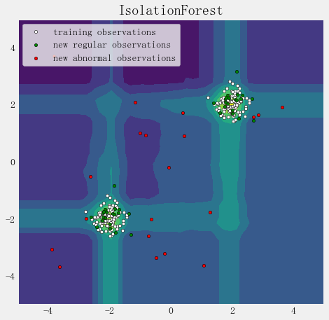
plt.title("IsolationForest")
plt.contourf(xx, yy, Z)  #cmap=plt.cm.Blues_r
b1 = plt.scatter(X_train[:, 0], X_train[:, 1], c='white', s=20, edgecolor='k')
b2 = plt.scatter(X_test[:, 0], X_test[:, 1], c='green', s=20, edgecolor='k')
c = plt.scatter(X_outliers[:, 0], X_outliers[:, 1], c='red', s=20, edgecolor='k')
plt.axis('tight')
plt.xlim((-5, 5))
plt.ylim((-5, 5))
plt.legend([b1, b2, c],
           ["training observations", "new regular observations", "new abnormal observations"],
           loc="upper left")
plt.show()

　　OneClassSVM

       One Class Learning 比较经典的算法是One-Class-SVM，这个算法的思路非常简单，就是寻找一个超平面将样本中的正例圈出来，预测就是用这个超平面做决策，在圈内的样本就认为是正样本。由于核函数计算比较耗时，在海量数据的场景用的并不多；

　　严格来说，OneCLassSVM不是一种outlier detection，而是一种novelty detection方法：它的训练集不应该掺杂异常点，因为模型可能会去匹配这些异常点。但在数据维度很高，或者对相关数据分布没有任何假设的情况下，OneClassSVM也可以作为一种很好的outlier detection方法。

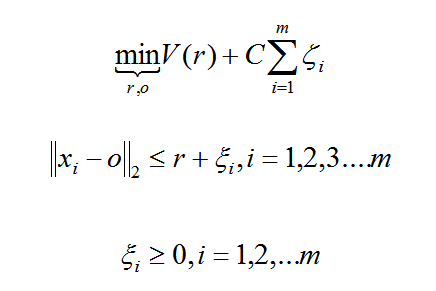
　　假设产生的超球体参数为中心 o 和对应的超球体半径 r >0，超球体体积V(r) 被最小化，中心 o 是支持行了的线性组合；跟传统SVM方法相似，可以要求所有训练数据点xi到中心的距离严格小于r。但是同时构造一个惩罚系数为 C 的松弛变量 ζ_i ,优化问题入下所示：

• 当训练集未被异常值污染时，该估计器最适合于新颖性检测；
• 高维中的离群检测，或者对上层数据的分布没有任何假设。

import numpy as np
import matplotlib.pyplot as plt
import matplotlib.font_manager
from sklearn import svm
 
# Generate train data
X = 0.3 * np.random.randn(100, 2)
X_train = np.r_[X + 2, X - 2]
X_test = np.r_[X + 2, X-2]
X_outliers = np.random.uniform(low=0.1, high=4, size=(20, 2))
#data = np.loadtxt('https://raw.githubusercontent.com/ffzs/dataset/master/outlier.txt', delimiter=' ')
#X_train = data[:900, :]
#X_test = data[-100:, :]

# 模型拟合
'''class sklearn.svm.OneClassSVM(kernel='rbf', degree=3, gamma=0.0, coef0=0.0, 
            tol=0.001, nu=0.5, shrinking=True, cache_size=200, 
            verbose=False, max_iter=-1, random_state=None)'''
clf = svm.OneClassSVM(nu=0.1, kernel='rbf', gamma=0.1)
clf.fit(X_train)

y_pred_train = clf.predict(X_train)
y_pred_test = clf.predict(X_test)
y_pred_outliers = clf.predict(X_outliers)
print ("novelty detection result:", y_pred_test)
n_error_train = y_pred_train[y_pred_train == -1].size
n_error_test = y_pred_test[y_pred_test == -1].size
n_error_outlier = y_pred_outliers[y_pred_outliers == 1].size
 
# plot the line , the points, and the nearest vectors to the plane
# 在平面中绘制点、线和距离平面最近的向量
#rand_mat = np.random.uniform(-1.0,1.0,(10000,5))  #np.random.randn(10000, 5)
#for i in range(X_train.shape[1]):
#    rand_mat[:,i] = (rand_mat[:,i]-X_train[:,i].mean()) * X_train[:,i].std()
#rand_mat = pd.DataFrame(rand_mat, columns=list('abcde'))
#rand_mat = rand_mat.sort_values(by = ['a','b'])
#rand_mat = rand_mat.values
#Z = clf.decision_function(rand_mat)
#xx = rand_mat[:,0].reshape((100,100))
#yy = rand_mat[:,1].reshape((100,100))
#xx, yy = np.meshgrid(np.linspace(X_train[:,0].min(), X_train[:,0].max(), 100), 
#                     np.linspace(X_train[:,1].min(), X_train[:,1].max(), 100))
#Z = clf.decision_function(np.c_[xx.ravel(), yy.ravel(), X_train[np.random.randint(900,size=10000),2:]])
xx, yy = np.meshgrid(np.linspace(-5, 5, 500), np.linspace(-5, 5, 500))
Z = clf.decision_function(np.c_[xx.ravel(), yy.ravel()])
Z = Z.reshape(xx.shape)
 
plt.title("Novelty Detection")
plt.contourf(xx, yy, Z, levels=np.linspace(Z.min(), 0, 7), cmap=plt.cm.PuBu)
a = plt.contour(xx, yy, Z, levels=[0, Z.max()], colors='palevioletred')
 
s = 40
b1 = plt.scatter(X_train[:, 0], X_train[:, 1], c='white', s=s, edgecolors='k')
b2 = plt.scatter(X_test[:, 0], X_test[:, 1], c='blueviolet', s=s, edgecolors='k')
c = plt.scatter(X_outliers[:, 0], X_outliers[:, 1], c='gold', s=s, edgecolors='k')
 
plt.axis('tight')
plt.xlim((-5, 5))
plt.ylim((-5, 5))
plt.legend([a.collections[0], b1, b2, c],
           ["learned frontier", 'training observations', "new regular observations", "new abnormal observations"],
           loc="upper left",
           prop=matplotlib.font_manager.FontProperties(size=11))
plt.xlabel(
    "error train: %d/200; errors novel regular: %d/40; errors novel abnormal:%d/40"%(
        n_error_train, n_error_test, n_error_outlier)    )
plt.show()

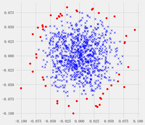
　　实际数据测试oneClassSVM

import numpy as np
import matplotlib.pyplot as plt
from numpy import genfromtxt
from sklearn import svm

#plt.style.use('fivethirtyeight')
 
def read_dataset(filePath, delimiter=','):
    return genfromtxt(filePath, delimiter=delimiter)
 
# use the same dataset
#tr_data = read_dataset('tr_data.csv')
tr_data = np.loadtxt('https://raw.githubusercontent.com/ffzs/dataset/master/outlier.txt', delimiter=' ')

'''
OneClassSVM(cache_size=200, coef0=0.0, degree=3, gamma=0.1, kernel='rbf',
      max_iter=-1, nu=0.05, random_state=None, shrinking=True, tol=0.001,
      verbose=False)
'''
clf = svm.OneClassSVM(nu=0.05, kernel='rbf', gamma=0.1)
clf.fit(tr_data[:,:2])
pred = clf.predict(tr_data[:,:2])
 
# inliers are labeled 1 , outliers are labeled -1
normal = tr_data[pred == 1]
abnormal = tr_data[pred == -1]
 
plt.plot(normal[:, 0], normal[:, 1], 'bx')
plt.plot(abnormal[:, 0], abnormal[:, 1], 'ro')

　　图片异常值检测OneClassSVM

import os
import cv2
from PIL import Image
 
def get_files(file_dir):
    for file in os.listdir(file_dir + '/AA475_B25'):
       A.append(file_dir + '/AA475_B25/' + file)
    length_A = len(os.listdir(file_dir + '/AA475_B25'))
    for file in range(length_A):
        img = Image.open(A[file])
        new_img = img.resize((128, 128))
        new_img = new_img.convert("L")
        matrix_img = np.asarray(new_img)
        AA.append(matrix_img.flatten())
    images1 = np.matrix(AA)
    return images1

　　

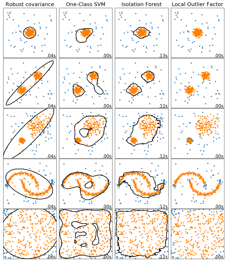
　　多种异常检测算法的比较

import time
import numpy as np
import matplotlib
import matplotlib.pyplot as plt
from sklearn import svm
from sklearn.datasets import make_blobs, make_moons
from sklearn.covariance import EllipticEnvelope
from sklearn.ensemble import IsolationForest
from sklearn.neighbors import LocalOutlierFactor
 
matplotlib.rcParams['contour.negative_linestyle'] = 'solid'
 
# Example settings
n_samples = 300
outliers_fraction = 0.15
n_outliers = int(outliers_fraction * n_samples)
n_inliers = n_samples - n_outliers
 
# define outlier/ anomaly detection methods to be compared
anomaly_algorithms = [
    ("Robust covariance", EllipticEnvelope(contamination=outliers_fraction)),
    ("One-Class SVM", svm.OneClassSVM(nu=outliers_fraction, kernel='rbf',gamma=0.1)),
    ("Isolation Forest", IsolationForest(behaviour='new', contamination=outliers_fraction, random_state=42)),
    ("Local Outlier Factor", LocalOutlierFactor(n_neighbors=35, contamination=outliers_fraction))
]
 
# define datasets
blobs_params = dict(random_state=0, n_samples=n_inliers, n_features=2)
datasets = [
    make_blobs(centers=[[0, 0], [0, 0]], cluster_std=0.5, **blobs_params)[0],
    make_blobs(centers=[[2, 2], [-2, -2]], cluster_std=[0.5, 0.5], **blobs_params)[0],
    make_blobs(centers=[[2, 2], [-2, -2]], cluster_std=[1.5, 0.3], **blobs_params)[0],
    4. * (make_moons(n_samples=n_samples, noise=0.05, random_state=0)[0] - np.array([0.5, 0.25])),
    14. * (np.random.RandomState(42).rand(n_samples, 2) - 0.5)
]
 
# Compare given classifiers under given settings
xx, yy = np.meshgrid(np.linspace(-7, 7, 150), np.linspace(-7, 7, 150))
 
plt.figure(figsize=(len(anomaly_algorithms) * 2 + 3, 12.5))
plt.subplots_adjust(left=0.02, right=0.98, bottom=0.001, top=0.96, wspace=0.05, hspace=0.01)
 
plot_num = 1
rng = np.random.RandomState(42)
 
 
for i_dataset, X in enumerate(datasets):
    # add outliers
    X = np.concatenate([X, rng.uniform(low=-6, high=6, size=(n_outliers, 2))], axis=0)
    for name, algorithm in anomaly_algorithms:
        print(name , algorithm)
        t0 = time.time()
        algorithm.fit(X)
        t1 = time.time()
        plt.subplot(len(datasets), len(anomaly_algorithms), plot_num)
        if i_dataset == 0:
            plt.title(name, size=18)
 
        # fit the data and tag outliers
        if name == 'Local Outlier Factor':
            y_pred = algorithm.fit_predict(X)
        else:
            y_pred = algorithm.fit(X).predict(X)
 
        # plot the levels lines and the points
        if name != "Local Outlier Factor":
            Z = algorithm.predict(np.c_[xx.ravel(), yy.ravel()])
            Z = Z.reshape(xx.shape)
            plt.contour(xx, yy, Z, levels=[0], linewidths=2, colors='black')
 
        colors = np.array(["#377eb8", '#ff7f00'])
        plt.scatter(X[:, 0], X[:, 1], s=10, color=colors[(y_pred + 1) // 2])
 
        plt.xlim(-7, 7)
        plt.ylim(-7, 7)
        plt.xticks(())
        plt.yticks(())
        plt.text(0.99, 0.01, ('%.2fs' % (t1 - t0)).lstrip('0'),
                 transform=plt.gca().transAxes, size=15,
                 horizontalalignment='right')
        plot_num += 1
 
plt.show()

 　　DBSCAN、BIRCH、LOF

# -*- coding: utf-8 -*-
"""
Created on Tue Jul 30 11:31:02 2019

@author: epsoft
"""

import time
import numpy as np
import pandas as pd
from sqlalchemy import create_engine
from sklearn.cluster import DBSCAN, Birch
from sklearn.neighbors import LocalOutlierFactor
from sklearn import metrics

import matplotlib
import matplotlib.pyplot as plt
matplotlib.rcParams['font.sans-serif'] = ['SimHei']
matplotlib.rcParams['font.family']='sans-serif'
matplotlib.rcParams['axes.unicode_minus'] = False

# ##############################################################################
# 获取数据
#数据库连接参数信息
config = {
        'username':'root',
        'passwd':'123',
        'host':'127.0.0.1',
        'port':'1521',
        'sid':'ORCL'
        }

engine = 'oracle://{username}:{passwd}@{host}:{port}/{sid}'.format(**config)  #dbname -- 各版本语法不同
db = create_engine(engine, encoding='utf-8')

sql = ''' 
        select hicode, max(hiname) as hiname, count(*) as counts, 
        sum(decode(sumfd_20,null,0,1))/count(*), --avg(sumfd_20), 
        sum(decode(sumfd_21,null,0,1))/count(*), --avg(sumfd_21), 
        sum(decode(sumfd_22,null,0,1))/count(*), --avg(sumfd_22), 
        sum(decode(sumfd_23,null,0,1))/count(*), --avg(sumfd_23), 
        sum(decode(sumfd_24,null,0,1))/count(*) --avg(sumfd_24) 
        from LU_CONSUMABLE_MATERIAL t 
        group by hicode
        having count(*) > 100
      '''
data = pd.read_sql_query(sql, db)
X = data.iloc[:,3:8].values

# ##############################################################################
# 参数设置
aa = []
for i in range(X.shape[0]-1):
    for j in range(i+1,X.shape[0]):
        aa.append(np.power(X[i]-X[j], 2).sum())
plt.hist(aa, bins=10, density=1, edgecolor ='k', facecolor='g', alpha=0.75)
plt.show()

# 调参
t0 = time.time()
optimum_parameter = [0,0,0]
for r in np.linspace(0.01, 0.1, 10):
    for min_samples in range(3,10):
        db = DBSCAN(eps=r, min_samples=min_samples).fit(X)
        score = metrics.silhouette_score(X, db.labels_)
        print('(%0.2f, %d) 轮廓系数: %0.3f'%(r, min_samples, score))
        if score > optimum_parameter[2]: optimum_parameter=[r, min_samples, score]
print('最佳参数为：eps=%0.2f, min_samples=%d, 轮廓系数=%0.3f'%(optimum_parameter[0], optimum_parameter[1], optimum_parameter[2]))
print('调参耗时：', time.time()-t0)

# ##############################################################################
# 调用密度聚类  DBSCAN
db = DBSCAN(eps=0.06, min_samples=5).fit(X)
# print(db.labels_)  # db.labels_为所有样本的聚类索引，没有聚类索引为-1
# print(db.core_sample_indices_) # 所有核心样本的索引

# 获取聚类个数。（聚类结果中-1表示没有聚类为离散点）
n_clusters_ = len(set(db.labels_)) - (1 if -1 in db.labels_ else 0)

# 异常样本标签
data.loc[db.labels_ == -1, 'hiname']


# 调用 Birch算法
branching_factor = 5
bi = Birch(threshold=0.06, branching_factor=branching_factor, n_clusters = None)
bi_outlier = bi.fit_predict(X)
from collections import Counter
aa = [i for i,c in Counter(bi_outlier).items() if c<branching_factor]
outlier_flag = np.array([i in aa for i in bi_outlier])
data.loc[outlier_flag, 'hiname']
plt.scatter(X[:, 0], X[:, 2], c=bi_outlier)
plt.show()


# 调用 LOF 算法
lof = LocalOutlierFactor(n_neighbors=5, contamination=0.04)  #contamination表示异常比例
lof_outlier = lof.fit_predict(X)
X_scores = lof.negative_outlier_factor_
radius = (X_scores.max() - X_scores) / (X_scores.max() - X_scores.min())

data.loc[lof_outlier == -1, 'hiname']
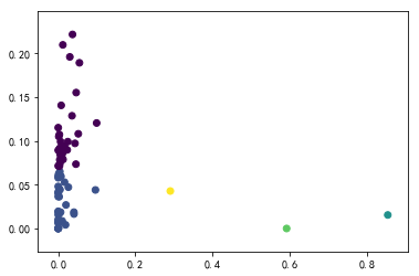
plt.scatter(X[:, 0], X[:, 2], c=lof_outlier)
#plt.plot(X[:, 0], X[:, 2], 'o')
plt.show()


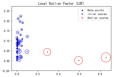
plt.scatter(X[:, 0], X[:, 2], color='k', s=3., label='Data points')
#plt.scatter(X[lof_outlier == -1, 0], X[lof_outlier == -1, 2], color='r', s=3., label='Outlier points')
plt.scatter(X[lof_outlier > -1, 0], X[lof_outlier > -1, 2], s=1000 * radius[lof_outlier > -1], edgecolors='b',
            facecolors='none', label='inlier scores')
plt.scatter(X[lof_outlier == -1, 0], X[lof_outlier == -1, 2], s=1000 * radius[lof_outlier == -1], edgecolors='r',
            facecolors='none', label='Outlier scores')
plt.axis('tight')
plt.xlim((min(X[:, 0])-0.05, max(X[:, 0])+0.05))
plt.ylim((min(X[:, 2])-0.05, max(X[:, 2])+0.05))
plt.title("Local Outlier Factor (LOF)")
#plt.xlabel("prediction errors: %d" % (n_errors))
legend = plt.legend(loc='upper right')
legend.legendHandles[0]._sizes = [10]
legend.legendHandles[1]._sizes = [20]
legend.legendHandles[2]._sizes = [20]
plt.show()


# ##############################################################################
# 模型评估
print('估计的聚类个数为: %d' % n_clusters_)
#print("同质性: %0.3f" % metrics.homogeneity_score(labels_true, db.labels_))  # 每个群集只包含单个类的成员。
#print("完整性: %0.3f" % metrics.completeness_score(labels_true, db.labels_))  # 给定类的所有成员都分配给同一个群集。
#print("V-measure: %0.3f" % metrics.v_measure_score(labels_true, db.labels_))  # 同质性和完整性的调和平均
#print("调整兰德指数: %0.3f" % metrics.adjusted_rand_score(labels_true, db.labels_))
#print("调整互信息: %0.3f" % metrics.adjusted_mutual_info_score(labels_true, db.labels_))
#print("Fowlkes-Mallows: %0.3f" % metrics.fowlkes_mallows_score(labels_true, db.labels_))
print("轮廓系数: %0.3f" % metrics.silhouette_score(X, db.labels_, metric='euclidean'))
print("Calinski-Harabasz分数: %0.3f" % metrics.calinski_harabaz_score(X, db.labels_))



# ##############################################################################
# 聚类结果可视化
from itertools import cycle
import matplotlib.pyplot as plt

plt.close('all')
plt.figure(figsize=(12,4))
plt.clf()

unique_labels = set(db.labels_)
core_samples_mask = np.zeros_like(db.labels_, dtype=bool)  # 设置一个样本个数长度的全false向量
core_samples_mask[db.core_sample_indices_] = True #将核心样本部分设置为true

# 使用黑色标注离散点
plt.subplot(121)
colors = [plt.cm.Spectral(each) for each in np.linspace(0, 1, len(unique_labels))]
for k, col in zip(unique_labels, colors):
    if k == -1:  # 聚类结果为-1的样本为离散点
        # 使用黑色绘制离散点
        col = [0, 0, 0, 1]

    class_member_mask = (db.labels_ == k)  # 将所有属于该聚类的样本位置置为true

    xy = X[class_member_mask & core_samples_mask]  # 将所有属于该类的核心样本取出，使用大图标绘制
    plt.plot(xy[:, 0], xy[:, 2], 'o', markerfacecolor=tuple(col),markeredgecolor='k', markersize=14)

    xy = X[class_member_mask & ~core_samples_mask]  # 将所有属于该类的非核心样本取出，使用小图标绘制
    plt.plot(xy[:, 0], xy[:, 2], 'o', markerfacecolor=tuple(col),markeredgecolor='k', markersize=6)

plt.title('对医院医疗耗材的异常值检测最佳聚类数: %d' % n_clusters_)
plt.xlabel(r'CQ类材料使用频率(%)')
plt.ylabel(r'单价200元以上CL类使用频率(%)')
#plt.show()


plt.subplot(122)
colors = cycle('bgrcmybgrcmybgrcmybgrcmy')
for k, col in zip(unique_labels, colors):
    class_member_mask = db.labels_ == k
    if k == -1:
        plt.plot(X[class_member_mask, 0], X[class_member_mask, 2], 'k' + '.')
    else:
        cluster_center = X[class_member_mask & core_samples_mask].mean(axis=0)
        plt.plot(X[class_member_mask, 0], X[class_member_mask, 2], col + '.')
        plt.plot(cluster_center[0], cluster_center[2], 'o', markerfacecolor=col,
                 markeredgecolor='k', markersize=14)
        for x in X[class_member_mask]:
            plt.plot([cluster_center[0], x[0]], [cluster_center[2], x[2]], col)

plt.title('Estimated number of clusters: %d' % n_clusters_)
plt.xlabel(r'CQ类材料使用频率(%)')
plt.ylabel(r'单价200元以上CL类使用频率(%)')
plt.show()

　

 　　模型评估格式化

def bench_k_means(estimator, name, data):
    t0 = time()
    estimator.fit(data)
    print('%-9s	%.2fs	%i	%.3f	%.3f	%.3f	%.3f	%.3f	%.3f'
          % (name, (time() - t0), estimator.inertia_,
             metrics.homogeneity_score(labels_true, estimator.labels_),
             metrics.completeness_score(labels_true, estimator.labels_),
             metrics.v_measure_score(labels_true, estimator.labels_),
             metrics.adjusted_rand_score(labels_true, estimator.labels_),
             metrics.adjusted_mutual_info_score(labels_true,  estimator.labels_,
                                                average_method='arithmetic'),
             metrics.silhouette_score(data, estimator.labels_,
                                      metric='euclidean',
                                      sample_size=sample_size)))

print(82 * '_')
print('init		time	inertia	homo	compl	v-meas	ARI	AMI	silhouette')
bench_k_means(KMeans(init='k-means++', n_clusters=n_digits, n_init=10), 
              name="k-means++", data=data)
bench_k_means(KMeans(init='random', n_clusters=n_digits, n_init=10),
              name="random", data=data)
pca = PCA(n_components=n_digits).fit(data)
bench_k_means(KMeans(init=pca.components_, n_clusters=n_digits, n_init=1),
              name="PCA-based",
              data=data)
print(82 * '_')

　　

 　　自编码器 

　　如果我们只有正样本数据，没有负样本数据，或者说只关注学习正样本的规律，那么利用正样本训练一个自编码器，编码器就相当于单分类的模型，对全量数据进行预测时，通过比较输入层和输出层的相似度就可以判断记录是否属于正样本。由于自编码采用神经网络实现，可以用GPU来进行加速计算，因此比较适合海量数据的场景。

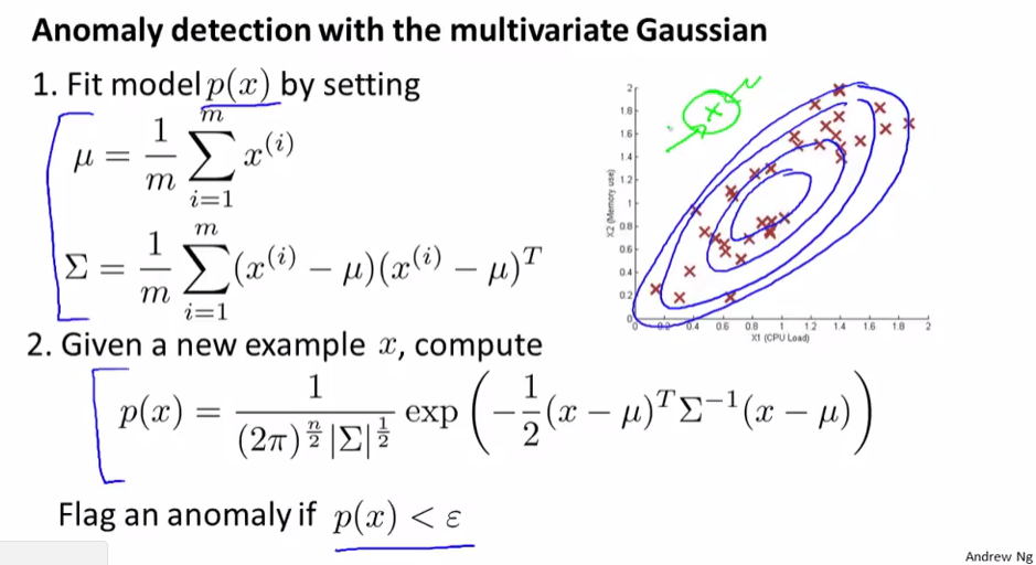
 　　多元高斯分布

参考链接：

Python机器学习笔记 异常点检测算法——Isolation Forest 

Python机器学习笔记——One Class SVM

异常点/离群点检测算法——LOF

新奇检测Novelty Detection

PAC在异常检测中的应用

TensorFlow中的变分自动编码器 VAE的tensorflow实现

异常检测: 应用多元高斯分布进行异常检测

机器学习（八）：AnomalyDetection异常检测_Python

异常检测的N种方法，阿里工程师都盘出来了

异常检测：百度是这样做的

 KPI异常检测挑战赛