以下内容参考CS231n。
上一篇关于分类器的文章,使用的是KNN分类器,KNN分类有两个主要的缺点:
- 空间上,需要存储所有的训练数据用于比较。
- 时间上,每次分类操作,需要和所有训练数据比较。
本文开始线性分类器的学习。
和KNN相比,线性分类器才算得上真正具有实用价值的分类器,也是后面神经网络和卷积神经网络的基础。
线性分类器中包括几个非常重要的部分:
- 权重矩阵W,偏差向量b
- 评分函数
- 损失函数
- 正则化
- 最优化
权重矩阵W (Weights)
- 可以理解为所有分类对应的模版向量w组成的矩阵,模版就是分类期望成为的样子。
- 训练数据可以理解为是N维空间中的一个向量v,v和W中每个模版做点积,点积越大,表示两个向量的夹角越小,也就越接近。
- 点积最大的模版w,就是v所对应的分类。
- W不是一直不变的。它会随着对损失函数最优化的过程,不断的调整。
偏差向量b (bias vector)
b是不是可以理解为,如果不设置b,那所有的分类线都要通过原点,那其实就起不到分类的作用了?
参考下图?三条线都通过原点,是无法对数据做分类的。
W和b分别对直线做旋转和平移。
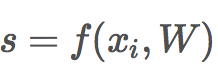
评分函数(score function)
![]()
之所以是线性分类器,就是因为评分函数使用线性方程计算分数。后面的神经网络会对线性函数做非线性处理。
下图直观的展示了分类器的线性。
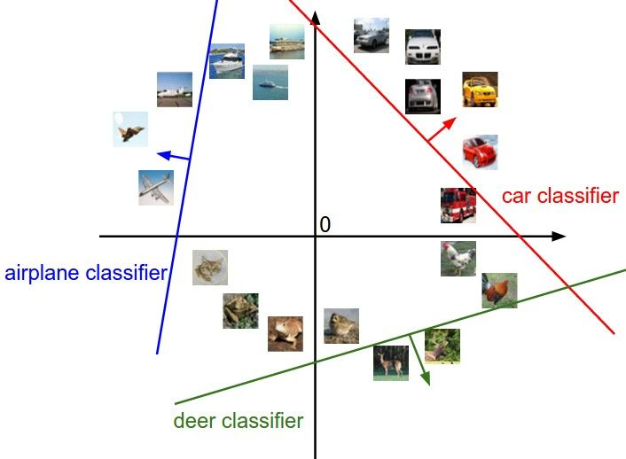
损失函数 (loss function)
如何判断当前的W和b是否合适,是否能够输出准确的分类?
通过损失函数,就可以计算预测的分类和实际分类之间的差异。通过不断减小损失函数的值,也就是减少差异,就可以得到对应的W和b。
Python实现
数据预处理
# 每行均值
mean_image = np.mean(X_train, axis=0)

# second: subtract the mean image from train and test data
# 零均值化,中心化,使数据分布在原点周围,可以加快训练的收敛速度
X_train -= mean_image
X_val -= mean_image
X_test -= mean_image
X_dev -= mean_image
处理b的技巧
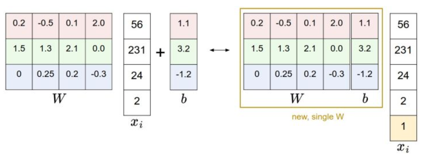
# third: append the bias dimension of ones (i.e. bias trick) so that our SVM
# only has to worry about optimizing a single weight matrix W.

# 技巧,将bias加到矩阵中,作为最后一列,直接参与矩阵运算。不用单独计算。
# hstack,水平地把数组的列组合起来
# 每行后面 加一个元素1

X_train = np.hstack([X_train, np.ones((X_train.shape[0], 1))])
X_val = np.hstack([X_val, np.ones((X_val.shape[0], 1))])
X_test = np.hstack([X_test, np.ones((X_test.shape[0], 1))])
X_dev = np.hstack([X_dev, np.ones((X_dev.shape[0], 1))])
计算损失函数
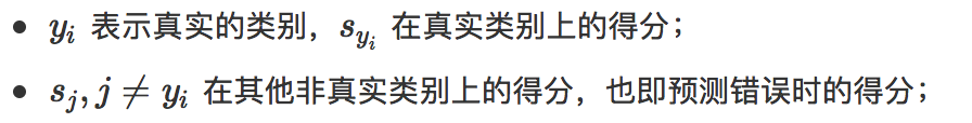
使用多类支持向量机作为损失函数。 SVM loss function,
 ,
, 
全体训练集上的平均损失值:
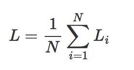
为了体现向量计算的高效,这里给出了非向量计算作为对比。
非向量版:
 1 # 多类支持向量机损失函数
 2 # SVM的损失函数想要SVM在正确分类上的得分始终比不正确分类上的得分高出一个边界值Delta
 3 # max(0, s1 - s2 + delta)
 4 # s1,错误分类, s2,正确分类
 5 def svm_loss_naive(W, X, y, reg):
 6
 7   # N, 500
 8   # D, 3073
 9   # C, 10
10   # W (3073, 10), 用(1,3073)左乘W,得到(1, 10)
11   # X(500, 3073), y(500,)
12
13   # 对W求导。 后面求使损失函数L减小的最快的w,也就是梯度下降最快的方向。
14   dW = np.zeros(W.shape) # initialize the gradient as zero
15
16   # compute the loss and the gradient
17   num_classes = W.shape[1] # 10
18   num_train = X.shape[0]     # 500
19   loss = 0.0
20   for i in range(num_train):
21     # 分数 = 点积
22     # 向量(1,D)和矩阵(D,C)的点积 = (1,C)    (c,)
23     # scores中的一行,表示所有类的打分
24     scores = X[i].dot(W)
25
26     # y[i],对的分类
27     correct_class_score = scores[y[i]]
28     for j in range(num_classes):
29       # 相等的分类不做处理
30       if j == y[i]:
31         continue
32       # 用其他分类的得分 - 最终分类的得分 + 1
33       margin = scores[j] - correct_class_score + 1 # note delta = 1
34
35       if margin > 0:
36         loss += margin
37
38         # (错的-对的),所以第一个是-X,第二个是X
39         # 500张图片的dW和,后面再除个500
40         dW[ :, y[i] ] += -X[ i, : ]
41         dW[ :, j ] += X[ i, : ]
42
43   loss /= num_train
44   dW /= num_train
45
46   # Add regularization to the loss.
47   # 正则化,https://blog.csdn.net/gsww404/article/details/80414675
48   # L2正则化
49   loss += reg * np.sum(W * W)
50
51   # 这里为什么不是2W
52   dW += reg * W
53
54   return loss, dW
向量版:
def svm_loss_vectorized(W, X, y, reg):
  loss = 0.0
  dW = np.zeros(W.shape) # initialize the gradient as zero

  num_classes = W.shape[1]
  num_train = X.shape[0]

  scores = X.dot(W) # (500, 10)
  correct_scores = scores[ np.arange(num_train),  y]  #(500, ),  取( 0~500, y[0~500])

  correct_scores = np.tile(correct_scores.reshape(num_train, 1) , (1, num_classes)) # (500, 10), 复制出10列,一行里的值是相同的
  margin = scores - correct_scores + 1

  margin[np.arange(num_train), y] = 0 # 正确的分类,不考虑
  margin[margin < 0] = 0          # 小于0的置为0,不考虑
  loss = np.sum(margin) / num_train
  loss += reg * np.sum(W * W)

  margin[ margin > 0 ] = 1  # 大于0的是造成损失的权重
  row_sum = np.sum( margin, axis = 1 ) # 对每行取和, dW[ :, y[i] ] += -X[ i, : ], 参考非向量的写法,每次遍历里,正确的分类都有被减一次
  margin[np.arange( num_train ), y] = -row_sum # 正确分类是负的,-X
  # 点积
  dW += np.dot(X.T, margin) / num_train + reg * W

  return loss, dW
随机初始化W,计算loss和gradient
# randn,高斯分布(正态分布)随机数
# 初始权重采用小一点的值
W = np.random.randn(3073, 10) * 0.0001

# grad,analytic gradient
loss, grad = svm_loss_naive(W, X_dev, y_dev, 0.000005)
检查梯度值的正确性。用数值梯度值(numerical gradient)和分析梯度值(analytic gradient)比较。
检查梯度方法:
def grad_check_sparse(f, x, analytic_grad, num_checks=10, h=1e-5):
  for i in range(num_checks):
    # 随机取一个位置
    ix = tuple([randrange(m) for m in x.shape])

    oldval = x[ix]
    x[ix] = oldval + h # increment by h
    fxph = f(x) # evaluate f(x + h)
    x[ix] = oldval - h # increment by h  # decrement ?
    fxmh = f(x) # evaluate f(x - h)
    x[ix] = oldval # reset

    # 对称差分
    grad_numerical = (fxph - fxmh) / (2 * h)
    grad_analytic = analytic_grad[ix]

    # 相对误差 ??
    rel_error = abs(grad_numerical - grad_analytic) / (abs(grad_numerical) + abs(grad_analytic))
比较分析梯度和数值梯度:
# 检查计算的梯度值是否正确
# Compute the loss and its gradient at W.
loss, grad = svm_loss_naive(W, X_dev, y_dev, 0.0)

# Numerically compute the gradient along several randomly chosen dimensions, and
# compare them with your analytically computed gradient. The numbers should match
# almost exactly along all dimensions.
from cs231n.gradient_check import grad_check_sparse
f = lambda w: svm_loss_naive(w, X_dev, y_dev, 0.0)[0] # 取loss
grad_numerical = grad_check_sparse(f, W, grad)

# do the gradient check once again with regularization turned on
# you didn't forget the regularization gradient did you?
loss, grad = svm_loss_naive(W, X_dev, y_dev, 5e1)
f = lambda w: svm_loss_naive(w, X_dev, y_dev, 5e1)[0]
grad_numerical = grad_check_sparse(f, W, grad)
创建一个线性分类器类
最优化方法使用 随机梯度下降法(SGD,Stochastic Gradient Descent)。
class LinearClassifier(object):

  def __init__(self):
    self.W = None

  # 训练,也是最优化,调参的过程。
  def train(self, X, y, learning_rate=1e-3, reg=1e-5, num_iters=100,
            batch_size=200, verbose=False):
    """
    Train this linear classifier using stochastic gradient descent.

    Inputs:
    - X: A numpy array of shape (N, D) containing training data; there are N
      training samples each of dimension D.
    - y: A numpy array of shape (N,) containing training labels; y[i] = c
      means that X[i] has label 0 <= c < C for C classes. C是所有类别吧?
    - learning_rate: (float) learning rate for optimization.
    - reg: (float) regularization strength.
    - num_iters: (integer) number of steps to take when optimizing
    - batch_size: (integer) number of training examples to use at each step.
    - verbose: (boolean) If true, print progress during optimization.

    Outputs:
    A list containing the value of the loss function at each training iteration.
    """
    num_train, dim = X.shape
    num_classes = np.max(y) + 1 # assume y takes values 0...K-1 where K is number of classes
    if self.W is None:
      self.W = 0.001 * np.random.randn(dim, num_classes)

    loss_history = []
    for it in range(num_iters):
      X_batch = None
      y_batch = None

      # 默认是replacement = true, 随机出来的数,还要再放回到样本池中
      randomRows = np.random.choice(num_train, batch_size)
      X_batch = X[randomRows]
      y_batch = y[randomRows]

      # evaluate loss and gradient
      loss, grad = self.loss(X_batch, y_batch, reg)
      loss_history.append(loss)

      # perform parameter update
      self.W += -learning_rate * grad

      if verbose and it % 100 == 0:
        print('iteration %d / %d: loss %f' % (it, num_iters, loss))

    return loss_history

  # 预测
  def predict(self, X):
    y_pred = np.zeros(X.shape[0])
    y_pred = np.argmax( np.dot( X, self.W ), axis=1 )

    return y_pred

  # 计算损失值
  def loss(self, X_batch, y_batch, reg):
    pass
继承基类LinearClassifier,定义SVM分类器
class LinearSVM(LinearClassifier):
  """ A subclass that uses the Multiclass SVM loss function """

  def loss(self, X_batch, y_batch, reg):
    return svm_loss_vectorized(self.W, X_batch, y_batch, reg)
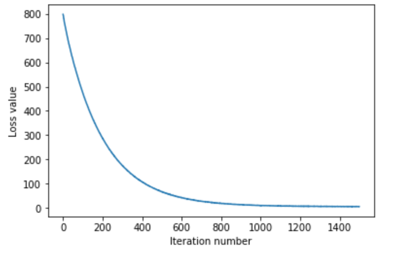
每次随机取出200个数据,训练1500次。 下图显示,损失值随着训练的迭代,追减降低。
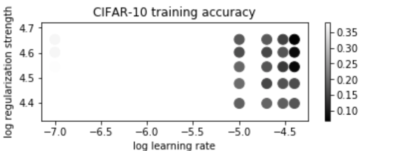
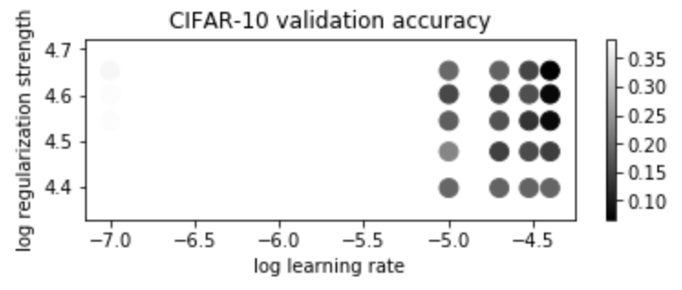
对于CIFAR-10的训练集和验证集的准确度如下。
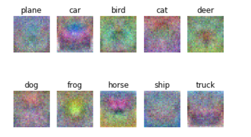
下图是最终训练出来的W所对应的图片。从图中可以看出最终的W,通过5万张图的训练, 提取出了具有指定分类的特征。
python相关:
- np.mean(a, axis=None),
- 计算平均值。 axis=0,对整列计算均值。
- np.hstack(tup),
- 在水平方向上合并
- np.vstack(tup),
- 在竖直方向上合并
- np.stack(arrays, axis=0),
- 增加了一个维度,而且合并的两个的形状必须一样。
- np.tile(A, reps),
- A是被重复的对象,reps是在不同维度上重复的次数
- np.random.randn,
- [0,1)范围内的随机数,满足高斯分布
- tuple([randrange(m) for m in x.shape]),
- 随机选择x中的任意位置
- f = lambda w: svm_loss_naive(w, X_dev, y_dev, 0.0)[0],
- lambda函数,w是参数,:后面是函数体。
- np.random.choice(a, size=None, replace=True, p=None),
- 从a中随机选择size个数。replace=True,表示随机取出的数,还要放回去。
- np.max(a, axis=None, out=None, keepdims=np._NoValue),
- 取最大值,也可以取每行或者每列中的最大值。
- np.argmax,
- 和np.max类似,区别是返回的是索引。
Reference:
1、知乎CS231n中文版,https://zhuanlan.zhihu.com/p/20918580?refer=intelligentunit