python数字图像处理（19）：骨架提取与分水岭算法

https://www.cnblogs.com/denny402/p/5167414.html

骨架提取与分水岭算法也属于形态学处理范畴，都放在morphology子模块内。

1、骨架提取

骨架提取，也叫二值图像细化。这种算法能将一个连通区域细化成一个像素的宽度，用于特征提取和目标拓扑表示。

morphology子模块提供了两个函数用于骨架提取，分别是Skeletonize（）函数和medial_axis（）函数。我们先来看Skeletonize（）函数。

格式为：skimage.morphology.skeletonize(image)

输入和输出都是一幅二值图像。

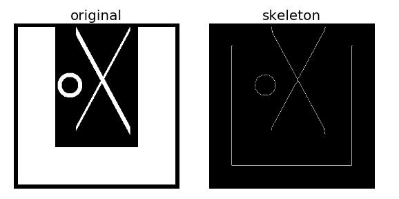
例1：

from skimage import morphology,draw
import numpy as np
import matplotlib.pyplot as plt

#创建一个二值图像用于测试
image = np.zeros((400, 400))

#生成目标对象1(白色U型)
image[10:-10, 10:100] = 1
image[-100:-10, 10:-10] = 1
image[10:-10, -100:-10] = 1

#生成目标对象2（X型）
rs, cs = draw.line(250, 150, 10, 280)
for i in range(10):
    image[rs + i, cs] = 1
rs, cs = draw.line(10, 150, 250, 280)
for i in range(20):
    image[rs + i, cs] = 1

#生成目标对象3（O型）
ir, ic = np.indices(image.shape)
circle1 = (ic - 135)**2 + (ir - 150)**2 < 30**2
circle2 = (ic - 135)**2 + (ir - 150)**2 < 20**2
image[circle1] = 1
image[circle2] = 0

#实施骨架算法
skeleton =morphology.skeletonize(image)

#显示结果
fig, (ax1, ax2) = plt.subplots(nrows=1, ncols=2, figsize=(8, 4))

ax1.imshow(image, cmap=plt.cm.gray)
ax1.axis('off')
ax1.set_title('original', fontsize=20)

ax2.imshow(skeleton, cmap=plt.cm.gray)
ax2.axis('off')
ax2.set_title('skeleton', fontsize=20)

fig.tight_layout()
plt.show()

生成一幅测试图像，上面有三个目标对象，分别进行骨架提取，结果如下：

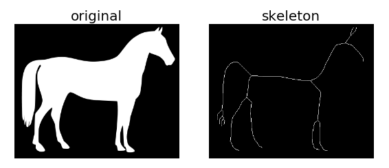
例2：利用系统自带的马图片进行骨架提取

from skimage import morphology,data,color
import matplotlib.pyplot as plt

image=color.rgb2gray(data.horse())
image=1-image #反相
#实施骨架算法
skeleton =morphology.skeletonize(image)

#显示结果
fig, (ax1, ax2) = plt.subplots(nrows=1, ncols=2, figsize=(8, 4))

ax1.imshow(image, cmap=plt.cm.gray)
ax1.axis('off')
ax1.set_title('original', fontsize=20)

ax2.imshow(skeleton, cmap=plt.cm.gray)
ax2.axis('off')
ax2.set_title('skeleton', fontsize=20)

fig.tight_layout()
plt.show()

medial_axis就是中轴的意思，利用中轴变换方法计算前景（1值）目标对象的宽度，格式为：

skimage.morphology.medial_axis(image, mask=None, return_distance=False)

mask: 掩模。默认为None, 如果给定一个掩模，则在掩模内的像素值才执行骨架算法。

return_distance: bool型值，默认为False. 如果为True, 则除了返回骨架，还将距离变换值也同时返回。这里的距离指的是中轴线上的所有点与背景点的距离。

import numpy as np
import scipy.ndimage as ndi
from skimage import morphology
import matplotlib.pyplot as plt

#编写一个函数，生成测试图像
def microstructure(l=256):
    n = 5
    x, y = np.ogrid[0:l, 0:l]
    mask = np.zeros((l, l))
    generator = np.random.RandomState(1)
    points = l * generator.rand(2, n**2)
    mask[(points[0]).astype(np.int), (points[1]).astype(np.int)] = 1
    mask = ndi.gaussian_filter(mask, sigma=l/(4.*n))
    return mask > mask.mean()

data = microstructure(l=64) #生成测试图像

#计算中轴和距离变换值
skel, distance =morphology.medial_axis(data, return_distance=True)

#中轴上的点到背景像素点的距离
dist_on_skel = distance * skel

fig, (ax1, ax2) = plt.subplots(1, 2, figsize=(8, 4))
ax1.imshow(data, cmap=plt.cm.gray, interpolation='nearest')
#用光谱色显示中轴
ax2.imshow(dist_on_skel, cmap=plt.cm.spectral, interpolation='nearest')
ax2.contour(data, [0.5], colors='w')  #显示轮廓线

fig.tight_layout()
plt.show()

2、分水岭算法

分水岭在地理学上就是指一个山脊，水通常会沿着山脊的两边流向不同的“汇水盆”。分水岭算法是一种用于图像分割的经典算法，是基于拓扑理论的数学形态学的分割方法。如果图像中的目标物体是连在一起的，则分割起来会更困难，分水岭算法经常用于处理这类问题，通常会取得比较好的效果。

分水岭算法可以和距离变换结合，寻找“汇水盆地”和“分水岭界限”，从而对图像进行分割。二值图像的距离变换就是每一个像素点到最近非零值像素点的距离，我们可以使用scipy包来计算距离变换。

在下面的例子中，需要将两个重叠的圆分开。我们先计算圆上的这些白色像素点到黑色背景像素点的距离变换，选出距离变换中的最大值作为初始标记点（如果是反色的话，则是取最小值），从这些标记点开始的两个汇水盆越集越大，最后相交于分山岭。从分山岭处断开，我们就得到了两个分离的圆。

例1：基于距离变换的分山岭图像分割

import numpy as np
import matplotlib.pyplot as plt
from scipy import ndimage as ndi
from skimage import morphology,feature

#创建两个带有重叠圆的图像
x, y = np.indices((80, 80))
x1, y1, x2, y2 = 28, 28, 44, 52
r1, r2 = 16, 20
mask_circle1 = (x - x1)**2 + (y - y1)**2 < r1**2
mask_circle2 = (x - x2)**2 + (y - y2)**2 < r2**2
image = np.logical_or(mask_circle1, mask_circle2)

#现在我们用分水岭算法分离两个圆
distance = ndi.distance_transform_edt(image) #距离变换
local_maxi =feature.peak_local_max(distance, indices=False, footprint=np.ones((3, 3)),
                            labels=image)   #寻找峰值
markers = ndi.label(local_maxi)[0] #初始标记点
labels =morphology.watershed(-distance, markers, mask=image) #基于距离变换的分水岭算法

fig, axes = plt.subplots(nrows=2, ncols=2, figsize=(8, 8))
axes = axes.ravel()
ax0, ax1, ax2, ax3 = axes

ax0.imshow(image, cmap=plt.cm.gray, interpolation='nearest')
ax0.set_title("Original")
ax1.imshow(-distance, cmap=plt.cm.jet, interpolation='nearest')
ax1.set_title("Distance")
ax2.imshow(markers, cmap=plt.cm.spectral, interpolation='nearest')
ax2.set_title("Markers")
ax3.imshow(labels, cmap=plt.cm.spectral, interpolation='nearest')
ax3.set_title("Segmented")

for ax in axes:
    ax.axis('off')

fig.tight_layout()
plt.show()

分水岭算法也可以和梯度相结合，来实现图像分割。一般梯度图像在边缘处有较高的像素值，而在其它地方则有较低的像素值，理想情况 下，分山岭恰好在边缘。因此，我们可以根据梯度来寻找分山岭。

例2：基于梯度的分水岭图像分割

import matplotlib.pyplot as plt
from scipy import ndimage as ndi
from skimage import morphology,color,data,filter

image =color.rgb2gray(data.camera())
denoised = filter.rank.median(image, morphology.disk(2)) #过滤噪声

#将梯度值低于10的作为开始标记点
markers = filter.rank.gradient(denoised, morphology.disk(5)) <10
markers = ndi.label(markers)[0]

gradient = filter.rank.gradient(denoised, morphology.disk(2)) #计算梯度
labels =morphology.watershed(gradient, markers, mask=image) #基于梯度的分水岭算法

fig, axes = plt.subplots(nrows=2, ncols=2, figsize=(6, 6))
axes = axes.ravel()
ax0, ax1, ax2, ax3 = axes

ax0.imshow(image, cmap=plt.cm.gray, interpolation='nearest')
ax0.set_title("Original")
ax1.imshow(gradient, cmap=plt.cm.spectral, interpolation='nearest')
ax1.set_title("Gradient")
ax2.imshow(markers, cmap=plt.cm.spectral, interpolation='nearest')
ax2.set_title("Markers")
ax3.imshow(labels, cmap=plt.cm.spectral, interpolation='nearest')
ax3.set_title("Segmented")

for ax in axes:
    ax.axis('off')

fig.tight_layout()
plt.show()