-
数据说明
本数据是一份汽车贷款违约数据
application_id 申请者ID
account_number 账户号
bad_ind 是否违约
vehicle_year 汽车购买时间
vehicle_make 汽车制造商
bankruptcy_ind 曾经破产标识
tot_derog 五年内信用不良事件数量(比如手机欠费消号)
tot_tr 全体账户数量
age_oldest_tr 最久账户存续时间(月)
tot_open_tr 在使用账户数量
tot_rev_debt 在使用可循环贷款帐户余额(比如信用卡欠款)
tot_rev_line 可循环贷款帐户限额(信用卡授权额度)
rev_util 可循环贷款帐户使用比例(余额/限额)
fico_score FICO打分
purch_price 汽车购买金额(元)
msrp 建议售价
down_pyt 分期付款的首次交款
loan_term 贷款期限(月)
loan_amt 贷款金额
ltv 贷款金额/建议售价*100
tot_income 月均收入(元)
veh_mileage 行使历程(Mile)
used_ind 是否二手车
weight 样本权重
-
导入数据和数据清洗
accepts<-read.csv("accepts.csv")
accepts<-na.omit(accepts)
attach(accepts)
-
分类变量的相关关系
曾经破产标识与是否违约是否有关系?
table(bankruptcy_ind,bad_ind)
对于两分类变量的列联表分析,使用prettyR包中的xtab函数,并进行卡方检验
library(prettyR)
xtab(~ bankruptcy_ind + bad_ind, data=accepts, chisq = TRUE)
-
逻辑回归
随机抽样,建立训练集与测试集
set.seed(100)
select<-sample(1:nrow(accepts),length(accepts$application_id)*0.7)
train=accepts[select,]
test=accepts[-select,]
attach(train)
R中的logit回归
lg<-glm(bad_ind ~fico_score+bankruptcy_ind+tot_derog+age_oldest_tr+rev_util+ltv+veh_mileage,family=binomial(link='logit'))
summary(lg)
lg_ms<-step(lg,direction = "both")
summary(lg_ms)
生成预测概率
train$p <- predict(lmg1,train,type = "response")
summary(train$p)
test$p<-predict(lmg1, test,type = "response")
-
模型评估
一.ROC指标
roc曲线:接收者操作特征(receiveroperating characteristic),roc曲线上每个点反映着对同一信号刺激的感受性。
横轴:负正类率(false postive rate FPR)特异度,划分实例中所有负例占所有负例的比例;(1-Specificity)
纵轴:真正类率(true postive rate TPR)灵敏度,Sensitivity(正类覆盖率)
2针对一个二分类问题,将实例分成正类(postive)或者负类(negative)。但是实际中分类时,会出现四种情况.
(1)若一个实例是正类并且被预测为正类,即为真正类(True Postive TP)
(2)若一个实例是正类,但是被预测成为负类,即为假负类(False Negative FN)
(3)若一个实例是负类,但是被预测成为正类,即为假正类(False Postive FP)
(4)若一个实例是负类,但是被预测成为负类,即为真负类(True Negative TN)
TP:正确的肯定数目
FN:漏报,没有找到正确匹配的数目
FP:误报,没有的匹配不正确
TN:正确拒绝的非匹配数目

由上表可得出横,纵轴的计算公式:
(1)真正类率(True Postive Rate)TPR: TP/(TP+FN),代表分类器预测的正类中实际正实例占所有正实例的比例。Sensitivity
(2)负正类率(False Postive Rate)FPR: FP/(FP+TN),代表分类器预测的正类中实际负实例占所有负实例的比例。1-Specificity
(3)真负类率(True Negative Rate)TNR: TN/(FP+TN),代表分类器预测的负类中实际负实例占所有负实例的比例,TNR=1-FPR。Specificity
假设采用逻辑回归分类器,其给出针对每个实例为正类的概率,那么通过设定一个阈值如0.6,概率大于等于0.6的为正类,小于0.6的为负类。对应的就可以算出一组(FPR,TPR),在平面中得到对应坐标点。随着阈值的逐渐减小,越来越多的实例被划分为正类,但是这些正类中同样也掺杂着真正的负实例,即TPR和FPR会同时增大。阈值最大时,对应坐标点为(0,0),阈值最小时,对应坐标点(1,1)。
如下面这幅图,(a)图中实线为ROC曲线,线上每个点对应一个阈值

横轴FPR:1-TNR,1-Specificity,FPR越大,预测正类中实际负类越多。
纵轴TPR:Sensitivity(正类覆盖率),TPR越大,预测正类中实际正类越多。
理想目标:TPR=1,FPR=0,即图中(0,1)点,故ROC曲线越靠拢(0,1)点,越偏离45度对角线越好,Sensitivity、Specificity越大效果越好。
二 如何画roc曲线
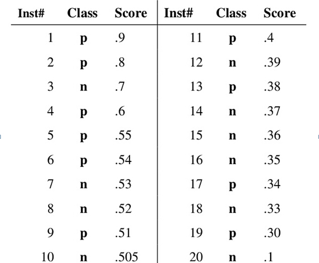
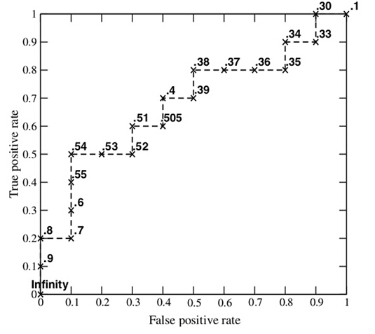
假设已经得出一系列样本被划分为正类的概率,然后按照大小排序,下图是一个示例,图中共有20个测试样本,“Class”一栏表示每个测试样本真正的标签(p表示正样本,n表示负样本),“Score”表示每个测试样本属于正样本的概率。
接下来,我们从高到低,依次将“Score”值作为阈值threshold,当测试样本属于正样本的概率大于或等于这个threshold时,我们认为它为正样本,否则为负样本。举例来说,对于图中的第4个样本,其“Score”值为0.6,那么样本1,2,3,4都被认为是正样本,因为它们的“Score”值都大于等于0.6,而其他样本则都认为是负样本。每次选取一个不同的threshold,我们就可以得到一组FPR和TPR,即ROC曲线上的一点。这样一来,我们一共得到了20组FPR和TPR的值,将它们画在ROC曲线的结果如下图:
AUC(Area under Curve):Roc曲线下的面积,介于0.1和1之间。Auc作为数值可以直观的评价分类器的好坏,值越大越好。
首先AUC值是一个概率值,当你随机挑选一个正样本以及负样本,当前的分类算法根据计算得到的Score值将这个正样本排在负样本前面的概率就是AUC值,AUC值越大,当前分类算法越有可能将正样本排在负样本前面,从而能够更好地分类。
三.用R代码画ROC曲线
install.packages("pROC")
library(pROC)
plot.roc(bad_ind~p,train,col="1")->r1
rocobjtr<- roc(train$bad_ind, train$p)
auc(rocobjtr)
lines.roc(bad_ind~p,test,col='2')->r2
rocobjte <- roc(test$bad_ind, test$p)
auc(rocobjte)
roc.test(r1,r2)

自定义函数画ROC曲线,提升图,洛伦兹图,以及KS曲线
plot_roc<-function(pred,actual,data_name='data',col='black',add=FALSE,pos=c(0.7,0.2)){
  library(ROCR)
  actual<-factor(actual)
  if(length(pred)!=length(actual)){
    stop("Pred and actual must have the same length")
  }
  if(length(levels(actual))!=2){
    stop("Only binary y supported")
  }
  index_set<-prediction(pred,actual)
  perf<-performance(index_set,'tpr','fpr')
  plot(perf,col=col,lty=2,
       lwd=2,
       add=add,
       main='ROC-Curve')
  abline(0,1,lty=2,col='red')
  auc <- performance(index_set,"auc")@y.values[[1]]
  lr_m_str<-paste0(data_name,"-AUC:",round(auc,4))
  text(pos[1],pos[2],lr_m_str)
}

plot_lift<-function(pred,actual,data_name='data',col='black',add=FALSE,pos=c(0.8,1.5)){
  library(ROCR)
  actual<-factor(actual)
  if(length(pred)!=length(actual)){
    stop("Pred and actual must have the same length")
  }
  if(length(levels(actual))!=2){
    stop("Only binary y supported")
  }
  index_set<-prediction(pred,actual)
  lift <- performance(index_set,measure='lift')@y.values[[1]]
  depth <- performance(index_set,measure='rpp')@y.values[[1]]
  if(add==FALSE){
    plot(depth,lift,type='l',col=col,
         lty=1,lwd=1,
         main='Lift-Curve')
  }
  else{
    lines(depth,lift,type='l',col=col,
          lty=1,lwd=1)
  }
  abline(h=1,lty=2,col='red')
  legend(pos[1],pos[2],data_name,fill=col,text.width=3)
}

plot_Lorenz<-function(pred,actual,data_name='data',col='black',add=FALSE,pos=c(0.8,0.1)){
  library(ROCR)
  actual<-factor(actual)
  if(length(pred)!=length(actual)){
    stop("Pred and actual must have the same length")
  }
  if(length(levels(actual))!=2){
    stop("Only binary y supported")
  }
  pred_Tr <- prediction(pred,actual)
  tpr <- performance(pred_Tr,measure='tpr')@y.values[[1]]
  depth <- performance(pred_Tr,measure='rpp')@y.values[[1]]
  if(add==FALSE){
    plot(depth,tpr,type='l',col=col,
         lty=1,lwd=1,
         main='Lorenz-Curve')
  }
  else{
    lines(depth,tpr,type='l',col=col,
          lty=1,lwd=1)
  }
  abline(0,1,lty=2,col='red')
  legend(pos[1],pos[2],data_name,fill=col,text.width=3)
}

plot_KS<-function(pred,actual,data_name='data',col='black',add=FALSE,pos=c(0.5,0.1)){
  library(ROCR)
  actual<-factor(actual)
  if(length(pred)!=length(actual)){
    stop("Pred and actual must have the same length")
  }
  if(length(levels(actual))!=2){
    stop("Only binary y supported")
  }
  pred_Tr <- prediction(pred,actual)
  depth <- performance(pred_Tr,measure='rpp')@y.values[[1]]
  tpr <- performance(pred_Tr,measure='tpr')@y.values[[1]]
  fpr <- performance(pred_Tr,measure='fpr')@y.values[[1]]
  ks<-(tpr-fpr)
  kslable<-paste0("KS:",max(ks))
  if(add==FALSE){
    plot(depth,ks,type='l',
         main='K-S-Curve',
         ylab='KS',xlab='depth')
    legend(pos[1],pos[2],paste0(kslable,'-',data_name),fill=col,text.width=3)
  }
  else{
    lines(depth,ks,type='l',col=col,
          lty=1,lwd=1)
    legend(pos[1],pos[2],paste0(kslable,'-',data_name),fill=col,text.width=3)
  }
}

thresholds<-function(pred,actual,method='best'){
  library(pROC)
  rocobjtr<- roc(actual,pred)
  thresholds<-rocobjtr$thresholds
  res<-coords(my_roc, method, ret = "threshold")
  return(res)
}

legend(0.3,0.2,paste('train:',auc(rocobjtr),sep=''),2:8)
legend(0.3,0.1,paste('test:',auc(rocobjte),sep=''),2:8)