Chapter 3 - Regression Models
Segment 3 - Logistic regression
Logistic Regression
Logistic regression is a simple machine learning method you can use to predict the value of a numeric categorical variable based on its relationship with predictor variables.
Logistic Regression Use Cases
- Customer Churn Prediction
- Employee Attrition Modeling
- Hazardous Event Prediction
- Purchase Propensity vs. Ad Spend Analysis
Logistic Regression Assumptions
- Data is free of missing values
- The predictant variable is binary(that is, it only accepts two values) or ordinal (that is, a categorical variable with ordered values)
- All predictors are independent of each other
- There are at least 50 observations per predictor variable (to ensure reliable results)
import numpy as np
import pandas as pd
import seaborn as sb
import matplotlib.pyplot as plt
import sklearn

from pandas import Series, DataFrame
from pylab import rcParams
from sklearn import preprocessing
from sklearn.linear_model import LogisticRegression
from sklearn.model_selection import train_test_split
from sklearn.model_selection import cross_val_predict

from sklearn import metrics
from sklearn.metrics import classification_report
from sklearn.metrics import confusion_matrix
from sklearn.metrics import precision_score, recall_score
%matplotlib inline
rcParams['figure.figsize'] = 5, 4
sb.set_style('whitegrid')
Logistic regression on the titanic dataset
address = '~/Data/titanic-training-data.csv'
titanic_training = pd.read_csv(address)
titanic_training.columns = ['PassengerId','Survived','Pclass','Name','Sex','Age','SibSp','Parch','Ticket','Fare','Cabin','Embarked']
print(titanic_training.head())
   PassengerId  Survived  Pclass
0            1         0       3
1            2         1       1
2            3         1       3
3            4         1       1
4            5         0       3

                                                Name     Sex   Age  SibSp
0                            Braund, Mr. Owen Harris    male  22.0      1
1  Cumings, Mrs. John Bradley (Florence Briggs Th...  female  38.0      1
2                             Heikkinen, Miss. Laina  female  26.0      0
3       Futrelle, Mrs. Jacques Heath (Lily May Peel)  female  35.0      1
4                           Allen, Mr. William Henry    male  35.0      0

   Parch            Ticket     Fare Cabin Embarked
0      0         A/5 21171   7.2500   NaN        S
1      0          PC 17599  71.2833   C85        C
2      0  STON/O2. 3101282   7.9250   NaN        S
3      0            113803  53.1000  C123        S
4      0            373450   8.0500   NaN        S
print(titanic_training.info())
<class 'pandas.core.frame.DataFrame'>
RangeIndex: 891 entries, 0 to 890
Data columns (total 12 columns):
 #   Column       Non-Null Count  Dtype
---  ------       --------------  -----
 0   PassengerId  891 non-null    int64
 1   Survived     891 non-null    int64
 2   Pclass       891 non-null    int64
 3   Name         891 non-null    object
 4   Sex          891 non-null    object
 5   Age          714 non-null    float64
 6   SibSp        891 non-null    int64
 7   Parch        891 non-null    int64
 8   Ticket       891 non-null    object
 9   Fare         891 non-null    float64
 10  Cabin        204 non-null    object
 11  Embarked     889 non-null    object
dtypes: float64(2), int64(5), object(5)
memory usage: 83.7+ KB
None
VARIABLE DESCRIPTIONS
Survived - Survival (0 = No; 1 = Yes)
Pclass - Passenger Class (1 = 1st; 2 = 2nd; 3 = 3rd)
Name - Name
Sex - Sex
Age - Age
SibSp - Number of Siblings/Spouses Aboard
Parch - Number of Parents/Children Aboard
Ticket - Ticket Number
Fare - Passenger Fare (British pound)
Cabin - Cabin
Embarked - Port of Embarkation (C = Cherbourg, France; Q = Queenstown, UK; S = Southampton - Cobh, Ireland)
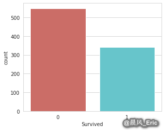
Checking that your target variable is binary
sb.countplot(x='Survived', data=titanic_training, palette='hls')
<matplotlib.axes._subplots.AxesSubplot at 0x7ff6fe9b95c0>
Checking for missing values
titanic_training.isnull().sum()
PassengerId      0
Survived         0
Pclass           0
Name             0
Sex              0
Age            177
SibSp            0
Parch            0
Ticket           0
Fare             0
Cabin          687
Embarked         2
dtype: int64
titanic_training.describe()
|
PassengerId |
Survived |
Pclass |
Age |
SibSp |
Parch |
Fare |
| count |
891.000000 |
891.000000 |
891.000000 |
714.000000 |
891.000000 |
891.000000 |
891.000000 |
| mean |
446.000000 |
0.383838 |
2.308642 |
29.699118 |
0.523008 |
0.381594 |
32.204208 |
| std |
257.353842 |
0.486592 |
0.836071 |
14.526497 |
1.102743 |
0.806057 |
49.693429 |
| min |
1.000000 |
0.000000 |
1.000000 |
0.420000 |
0.000000 |
0.000000 |
0.000000 |
| 25% |
223.500000 |
0.000000 |
2.000000 |
20.125000 |
0.000000 |
0.000000 |
7.910400 |
| 50% |
446.000000 |
0.000000 |
3.000000 |
28.000000 |
0.000000 |
0.000000 |
14.454200 |
| 75% |
668.500000 |
1.000000 |
3.000000 |
38.000000 |
1.000000 |
0.000000 |
31.000000 |
| max |
891.000000 |
1.000000 |
3.000000 |
80.000000 |
8.000000 |
6.000000 |
512.329200 |
Taking care of missing values
Dropping missing values
So let's just go ahead and drop all the variables that aren't relevant for predicting survival. We should at least keep the following:
- Survived - This variable is obviously relevant.
- Pclass - Does a passenger's class on the boat affect their survivability?
- Sex - Could a passenger's gender impact their survival rate?
- Age - Does a person's age impact their survival rate?
- SibSp - Does the number of relatives on the boat (that are siblings or a spouse) affect a person survivability? Probability
- Parch - Does the number of relatives on the boat (that are children or parents) affect a person survivability? Probability
- Fare - Does the fare a person paid effect his survivability? Maybe - let's keep it.
- Embarked - Does a person's point of embarkation matter? It depends on how the boat was filled... Let's keep it.
What about a person's name, ticket number, and passenger ID number? They're irrelavant for predicting survivability. And as you recall, the cabin variable is almost all missing values, so we can just drop all of these.
titanic_data = titanic_training.drop(['Name','Ticket','Cabin'], axis=1)
titanic_data.head()
|
PassengerId |
Survived |
Pclass |
Sex |
Age |
SibSp |
Parch |
Fare |
Embarked |
| 0 |
1 |
0 |
3 |
male |
22.0 |
1 |
0 |
7.2500 |
S |
| 1 |
2 |
1 |
1 |
female |
38.0 |
1 |
0 |
71.2833 |
C |
| 2 |
3 |
1 |
3 |
female |
26.0 |
0 |
0 |
7.9250 |
S |
| 3 |
4 |
1 |
1 |
female |
35.0 |
1 |
0 |
53.1000 |
S |
| 4 |
5 |
0 |
3 |
male |
35.0 |
0 |
0 |
8.0500 |
S |
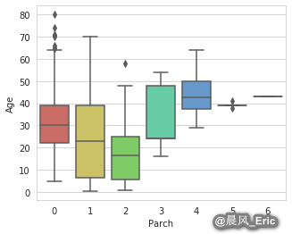
Imputing missing values
sb.boxplot(x='Parch', y='Age', data=titanic_data, palette='hls')
<matplotlib.axes._subplots.AxesSubplot at 0x7ff6fc140828>
Parch_groups = titanic_data.groupby(titanic_data['Parch'])
Parch_groups.mean()
|
PassengerId |
Survived |
Pclass |
Age |
SibSp |
Fare |
| Parch |
|
|
|
|
|
|
| 0 |
445.255162 |
0.343658 |
2.321534 |
32.178503 |
0.237463 |
25.586774 |
| 1 |
465.110169 |
0.550847 |
2.203390 |
24.422000 |
1.084746 |
46.778180 |
| 2 |
416.662500 |
0.500000 |
2.275000 |
17.216912 |
2.062500 |
64.337604 |
| 3 |
579.200000 |
0.600000 |
2.600000 |
33.200000 |
1.000000 |
25.951660 |
| 4 |
384.000000 |
0.000000 |
2.500000 |
44.500000 |
0.750000 |
84.968750 |
| 5 |
435.200000 |
0.200000 |
3.000000 |
39.200000 |
0.600000 |
32.550000 |
| 6 |
679.000000 |
0.000000 |
3.000000 |
43.000000 |
1.000000 |
46.900000 |
def age_approx(cols):
    Age = cols[0]
    Parch = cols[1]

    if pd.isnull(Age):
        if Parch == 0:
            return 32
        elif Parch == 1:
            return 24
        elif Parch == 2:
            return 17
        elif Parch == 3:
            return 33
        elif Parch == 4:
            return 45
        else:
            return 30
    else:
        return Age
titanic_data['Age'] = titanic_data[['Age','Parch']].apply(age_approx, axis=1)
titanic_data.isnull().sum()
PassengerId    0
Survived       0
Pclass         0
Sex            0
Age            0
SibSp          0
Parch          0
Fare           0
Embarked       2
dtype: int64
titanic_data.dropna(inplace=True)
titanic_data.reset_index(inplace=True, drop=True)

print(titanic_data.info())
<class 'pandas.core.frame.DataFrame'>
RangeIndex: 889 entries, 0 to 888
Data columns (total 9 columns):
 #   Column       Non-Null Count  Dtype
---  ------       --------------  -----
 0   PassengerId  889 non-null    int64
 1   Survived     889 non-null    int64
 2   Pclass       889 non-null    int64
 3   Sex          889 non-null    object
 4   Age          889 non-null    float64
 5   SibSp        889 non-null    int64
 6   Parch        889 non-null    int64
 7   Fare         889 non-null    float64
 8   Embarked     889 non-null    object
dtypes: float64(2), int64(5), object(2)
memory usage: 62.6+ KB
None
Converting categorical variables to a dummy indicators
from sklearn.preprocessing import LabelEncoder
label_encoder = LabelEncoder()
gender_cat = titanic_data['Sex']
gender_encoded = label_encoder.fit_transform(gender_cat)
gender_encoded[0:5]
array([1, 0, 0, 0, 1])
titanic_data.head()
|
PassengerId |
Survived |
Pclass |
Sex |
Age |
SibSp |
Parch |
Fare |
Embarked |
| 0 |
1 |
0 |
3 |
male |
22.0 |
1 |
0 |
7.2500 |
S |
| 1 |
2 |
1 |
1 |
female |
38.0 |
1 |
0 |
71.2833 |
C |
| 2 |
3 |
1 |
3 |
female |
26.0 |
0 |
0 |
7.9250 |
S |
| 3 |
4 |
1 |
1 |
female |
35.0 |
1 |
0 |
53.1000 |
S |
| 4 |
5 |
0 |
3 |
male |
35.0 |
0 |
0 |
8.0500 |
S |
# 1 = male / 0 = female
gender_DF = pd.DataFrame(gender_encoded, columns=['male_gender'])
gender_DF.head()
|
male_gender |
| 0 |
1 |
| 1 |
0 |
| 2 |
0 |
| 3 |
0 |
| 4 |
1 |
embarked_cat = titanic_data['Embarked']
embarked_encoded = label_encoder.fit_transform(embarked_cat)
embarked_encoded[0:100]
array([2, 0, 2, 2, 2, 1, 2, 2, 2, 0, 2, 2, 2, 2, 2, 2, 1, 2, 2, 0, 2, 2,
       1, 2, 2, 2, 0, 2, 1, 2, 0, 0, 1, 2, 0, 2, 0, 2, 2, 0, 2, 2, 0, 0,
       1, 2, 1, 1, 0, 2, 2, 2, 0, 2, 0, 2, 2, 0, 2, 2, 0, 2, 2, 0, 0, 2,
       2, 2, 2, 2, 2, 2, 0, 2, 2, 2, 2, 2, 2, 2, 2, 1, 2, 2, 2, 2, 2, 2,
       2, 2, 2, 2, 2, 2, 2, 0, 0, 2, 2, 2])
from sklearn.preprocessing import OneHotEncoder
binary_encoder = OneHotEncoder(categories='auto')
embarked_1hot = binary_encoder.fit_transform(embarked_encoded.reshape(-1,1))
embarked_1hot_mat = embarked_1hot.toarray()
embarked_DF = pd.DataFrame(embarked_1hot_mat, columns = ['C','Q','S'])
embarked_DF.head()
|
C |
Q |
S |
| 0 |
0.0 |
0.0 |
1.0 |
| 1 |
1.0 |
0.0 |
0.0 |
| 2 |
0.0 |
0.0 |
1.0 |
| 3 |
0.0 |
0.0 |
1.0 |
| 4 |
0.0 |
0.0 |
1.0 |
titanic_data.drop(['Sex','Embarked'], axis=1, inplace=True)
titanic_data.head()
|
PassengerId |
Survived |
Pclass |
Age |
SibSp |
Parch |
Fare |
| 0 |
1 |
0 |
3 |
22.0 |
1 |
0 |
7.2500 |
| 1 |
2 |
1 |
1 |
38.0 |
1 |
0 |
71.2833 |
| 2 |
3 |
1 |
3 |
26.0 |
0 |
0 |
7.9250 |
| 3 |
4 |
1 |
1 |
35.0 |
1 |
0 |
53.1000 |
| 4 |
5 |
0 |
3 |
35.0 |
0 |
0 |
8.0500 |
titanic_dmy = pd.concat([titanic_data, gender_DF, embarked_DF], axis=1, verify_integrity=True).astype(float)
titanic_dmy[0:5]
|
PassengerId |
Survived |
Pclass |
Age |
SibSp |
Parch |
Fare |
male_gender |
C |
Q |
S |
| 0 |
1.0 |
0.0 |
3.0 |
22.0 |
1.0 |
0.0 |
7.2500 |
1.0 |
0.0 |
0.0 |
1.0 |
| 1 |
2.0 |
1.0 |
1.0 |
38.0 |
1.0 |
0.0 |
71.2833 |
0.0 |
1.0 |
0.0 |
0.0 |
| 2 |
3.0 |
1.0 |
3.0 |
26.0 |
0.0 |
0.0 |
7.9250 |
0.0 |
0.0 |
0.0 |
1.0 |
| 3 |
4.0 |
1.0 |
1.0 |
35.0 |
1.0 |
0.0 |
53.1000 |
0.0 |
0.0 |
0.0 |
1.0 |
| 4 |
5.0 |
0.0 |
3.0 |
35.0 |
0.0 |
0.0 |
8.0500 |
1.0 |
0.0 |
0.0 |
1.0 |
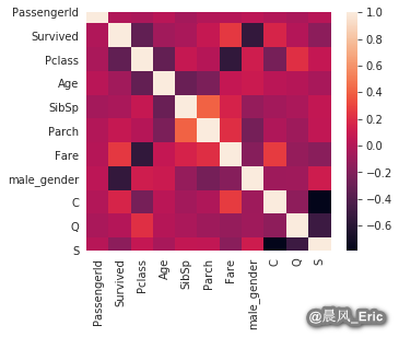
Checking for independence between features
sb.heatmap(titanic_dmy.corr())
<matplotlib.axes._subplots.AxesSubplot at 0x7ff6fc071dd8>
titanic_dmy.drop(['Fare','Pclass'], axis=1, inplace=True)
titanic_dmy.head()
|
PassengerId |
Survived |
Age |
SibSp |
Parch |
male_gender |
C |
Q |
S |
| 0 |
1.0 |
0.0 |
22.0 |
1.0 |
0.0 |
1.0 |
0.0 |
0.0 |
1.0 |
| 1 |
2.0 |
1.0 |
38.0 |
1.0 |
0.0 |
0.0 |
1.0 |
0.0 |
0.0 |
| 2 |
3.0 |
1.0 |
26.0 |
0.0 |
0.0 |
0.0 |
0.0 |
0.0 |
1.0 |
| 3 |
4.0 |
1.0 |
35.0 |
1.0 |
0.0 |
0.0 |
0.0 |
0.0 |
1.0 |
| 4 |
5.0 |
0.0 |
35.0 |
0.0 |
0.0 |
1.0 |
0.0 |
0.0 |
1.0 |
Checking that your dataset size is sufficient
titanic_dmy.info()
<class 'pandas.core.frame.DataFrame'>
RangeIndex: 889 entries, 0 to 888
Data columns (total 9 columns):
 #   Column       Non-Null Count  Dtype
---  ------       --------------  -----
 0   PassengerId  889 non-null    float64
 1   Survived     889 non-null    float64
 2   Age          889 non-null    float64
 3   SibSp        889 non-null    float64
 4   Parch        889 non-null    float64
 5   male_gender  889 non-null    float64
 6   C            889 non-null    float64
 7   Q            889 non-null    float64
 8   S            889 non-null    float64
dtypes: float64(9)
memory usage: 62.6 KB
X_train, X_test, y_train, y_test = train_test_split(titanic_dmy.drop('Survived',axis=1),
                                                   titanic_dmy['Survived'],test_size=0.2,
                                                   random_state=200)
print(X_train.shape)
print(y_train.shape)
(711, 8)
(711,)
X_train[0:5]
|
PassengerId |
Age |
SibSp |
Parch |
male_gender |
C |
Q |
S |
| 719 |
721.0 |
6.0 |
0.0 |
1.0 |
0.0 |
0.0 |
0.0 |
1.0 |
| 165 |
167.0 |
24.0 |
0.0 |
1.0 |
0.0 |
0.0 |
0.0 |
1.0 |
| 879 |
882.0 |
33.0 |
0.0 |
0.0 |
1.0 |
0.0 |
0.0 |
1.0 |
| 451 |
453.0 |
30.0 |
0.0 |
0.0 |
1.0 |
1.0 |
0.0 |
0.0 |
| 181 |
183.0 |
9.0 |
4.0 |
2.0 |
1.0 |
0.0 |
0.0 |
1.0 |
Deploying and evaluating the model
LogReg = LogisticRegression(solver='liblinear')
LogReg.fit(X_train, y_train)
LogisticRegression(solver='liblinear')
y_pred = LogReg.predict(X_test)
Model Evaluation
Classification report without cross-validation
print(classification_report(y_test, y_pred))
              precision    recall  f1-score   support

         0.0       0.83      0.88      0.85       109
         1.0       0.79      0.71      0.75        69

    accuracy                           0.81       178
   macro avg       0.81      0.80      0.80       178
weighted avg       0.81      0.81      0.81       178
K-fold cross-validation & confusion matrices
y_train_pred = cross_val_predict(LogReg, X_train, y_train, cv=5)
confusion_matrix(y_train, y_train_pred)
array([[377,  63],
       [ 91, 180]])
precision_score(y_train, y_train_pred)
0.7407407407407407
Make a test prediction
titanic_dmy[863:864]
|
PassengerId |
Survived |
Age |
SibSp |
Parch |
male_gender |
C |
Q |
S |
| 863 |
866.0 |
1.0 |
42.0 |
0.0 |
0.0 |
0.0 |
0.0 |
0.0 |
1.0 |
test_passenger = np.array([866,40,0,0,0,0,0,1]).reshape(1,-1)

print(LogReg.predict(test_passenger))
print(LogReg.predict_proba(test_passenger))
[1.]
[[0.26351831 0.73648169]]