TensorFlow Ops
1. Fun with TensorBoard
In TensorFlow, you collectively call constants, variables, operators as ops. TensorFlow is not just a software library, but a suite of softwares that include TensorFlow, TensorBoard, and Tensor Serving. To make the most out of TensorFlow, we should know how to use all of the above in conjunction with one another. In the first part of this lecture, we will explore TensorBoard.
TensorBoard is a graph visualization software included with any standard TensorFlow installation. In Google's own words:
"The computations you'll use TensorFlow for - like training a massive deep neural network - can be complex and confusing. To make it easier to understand, debug, and optimize TensorFlow programs, we've included a suite of visualization tools called TensorBoard."
TensorBoard, when fully configured, will look something like this.

When a user perform certain operations in a TensorBoard-activated TensorFlow program, these operations are exported to an event log file. TensorBoard is able to convert these event files to visualizations that can give insight into a model's graph and its runtime behavior. Learning to use TensorBoard early and often will make working with TensorFlow that much more enjoyable and productive.
Let's write your first TensorFlow program and visualize its computation graph with TensorBoard.
|
import tensorflow as tf a = tf.constant(2) b = tf.constant(3) x = tf.add(a, b) with tf.Session() as sess: print(sess.run(x)) |
To visualize the program with TensorBoard, we need to write log files of the program. To write event files, we first need to create a writer for those logs, using this code:
|
writer = tf.summary.FileWriter([logdir], [graph]) |
[graph] is the graph of the program you are working on. You can either call it using tf.get_default_graph(), which returns the default graph of the program, or through sess.graph, which returns the graph the session is handling. The latter requires you to already have created a session. Either way, make sure to create a writer only after you've defined your graph, else the graph visualized on TensorBoard would be incomplete.
[logdir] is the folder where you want to store those log files. You can choose [logdir] to be something meaningful such as './graphs' or './graphs/lecture02'.
|
import tensorflow as tf a = tf.constant(2) b = tf.constant(3) x = tf.add(a, b) writer = tf.summary.FileWriter('./graphs', tf.get_default_graph()) with tf.Session() as sess: # writer = tf.summary.FileWriter('./graphs', sess.graph) # if you prefer creating your writer using session's graph print(sess.run(x)) writer.close() |
Next, go to Terminal, run the program. Make sure that your present working directory is the same as where you ran your Python code.
|
$ python3 [my_program.py] $ tensorboard --logdir="./graphs" --port 6006 |
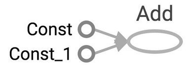
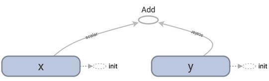
Open your browser and go to http://localhost:6006/ (or the port of your choice), you will see the TensorBoard page. Go to the Graph tab and you can verify that the graph indeed has 3 nodes, two constants and an Add op.
|
a = tf.constant(2) b = tf.constant(3) x = tf.add(a, b) |
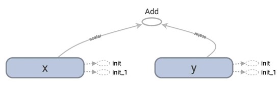
"Const" and "Const_1" correspond to a and b, and the node "Add" corresponds to x. The names we give them (a, b, and x) are for us to access them when we write code. They mean nothing for the internal TensorFlow. To make TensorBoard understand the names of your ops, you have to explicitly name them.
|
a = tf.constant(2, name="a") b = tf.constant(2, name="b") x = tf.add(a, b, name="add") |
Now if you run TensorBoard again, you see this graph:

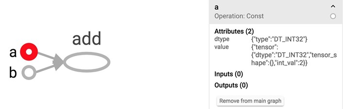
The graph itself defines the ops and dependencies. To see the value as well as the type of a node, simply click on that node:
Note: If you've run your code several times, there will be multiple event files in your [logdir]. TF will show only the latest graph and display the warning of multiple event files. To get rid of the warning, delete the event files you no longer need.
Of course, TensorBoard can do much more than just visualizing your graphs. During the course of the class, we will explore some most important functionalities of it.
2. Constant op
It's straightforward to create a constant in TensorFlow. We've already done it several times.
|
tf.constant(value, dtype=None, shape=None, name='Const', verify_shape=False) # constant of 1d tensor (vector) a = tf.constant([2, 2], name="vector") # constant of 2x2 tensor (matrix) b = tf.constant([[0, 1], [2, 3]], name="matrix") |
You can create a tensor of a specific dimension and fill it with a specific value, similar to Numpy.
|
tf.zeros(shape, dtype=tf.float32, name=None) # create a tensor of shape and all elements are zeros tf.zeros([2, 3], tf.int32) ==> [[0, 0, 0], [0, 0, 0]] |
|
tf.zeros_like(input_tensor, dtype=None, name=None, optimize=True) # create a tensor of shape and type (unless type is specified) as the input_tensor but all elements are zeros. # input_tensor [[0, 1], [2, 3], [4, 5]] tf.zeros_like(input_tensor) ==> [[0, 0], [0, 0], [0, 0]] |
|
tf.ones(shape, dtype=tf.float32, name=None) # create a tensor of shape and all elements are ones tf.ones([2, 3], tf.int32) ==> [[1, 1, 1], [1, 1, 1]] |
|
tf.ones_like(input_tensor, dtype=None, name=None, optimize=True) # create a tensor of shape and type (unless type is specified) as the input_tensor but all elements are ones. # input_tensor is [[0, 1], [2, 3], [4, 5]] tf.ones_like(input_tensor) ==> [[1, 1], [1, 1], [1, 1]] |
|
tf.fill(dims, value, name=None) # create a tensor filled with a scalar value. tf.fill([2, 3], 8) ==> [[8, 8, 8], [8, 8, 8]] |
You can create constants that are sequences
|
tf.lin_space(start, stop, num, name=None) # create a sequence of num evenly-spaced values are generated beginning at start. If num > 1, the values in the sequence increase by (stop - start) / (num - 1), so that the last one is exactly stop. # comparable to but slightly different from numpy.linspace tf.lin_space(10.0, 13.0, 4, name="linspace") ==> [10.0 11.0 12.0 13.0] |
|
tf.range([start], limit=None, delta=1, dtype=None, name='range') # create a sequence of numbers that begins at start and extends by increments of delta up to but not including limit # slight different from range in Python # 'start' is 3, 'limit' is 18, 'delta' is 3 tf.range(start, limit, delta) ==> [3, 6, 9, 12, 15] # 'start' is 3, 'limit' is 1, 'delta' is -0.5 tf.range(start, limit, delta) ==> [3, 2.5, 2, 1.5] # 'limit' is 5 tf.range(limit) ==> [0, 1, 2, 3, 4] |
Note that unlike NumPy or Python sequences, TensorFlow sequences are not iterable.
|
for _ in np.linspace(0, 10, 4): # OK for _ in tf.linspace(0.0, 10.0, 4): # TypeError: 'Tensor' object is not iterable. for _ in range(4): # OK for _ in tf.range(4): # TypeError: 'Tensor' object is not iterable. |
You can also generate random constants from certain distributions. See details.
|
tf.random_normal tf.truncated_normal tf.random_uniform tf.random_shuffle tf.random_crop tf.multinomial tf.random_gamma tf.set_random_seed |
3. Math Operations
TensorFlow math ops are pretty standard. You can visit the full list here. There are a few things that seem a bit tricky.
TensorFlow's zillion operations for division
The last time I checked, TensorFlow has 7 different div operations, all doing more or less the same thing: tf.div, tf.divide, tf.truediv, tf.floordiv, tf.realdiv, tf.truncateddiv, tf.floor_div. The person who created those ops must really like dividing numbers. Make sure you read the documentation to understand which one to use. At a high level, tf.div does TensorFlow's style division, while tf.divide does exactly Python's style division.
|
a = tf.constant([2, 2], name='a') b = tf.constant([[0, 1], [2, 3]], name='b') with tf.Session() as sess: print(sess.run(tf.div(b, a))) ⇒ [[0 0] [1 1]] print(sess.run(tf.divide(b, a))) ⇒ [[0. 0.5] [1. 1.5]] print(sess.run(tf.truediv(b, a))) ⇒ [[0. 0.5] [1. 1.5]] print(sess.run(tf.floordiv(b, a))) ⇒ [[0 0] [1 1]] print(sess.run(tf.realdiv(b, a))) ⇒ # Error: only works for real values print(sess.run(tf.truncatediv(b, a))) ⇒ [[0 0] [1 1]] print(sess.run(tf.floor_div(b, a))) ⇒ [[0 0] [1 1]] |
tf.add_n
Allows you to add multiple tensors.
tf.add_n([a, b, b]) => equivalent to a + b + b
Dot product in TensorFlow
Note that tf.matmul no longer does dot product. It multiplies matrices of ranks greater or equal to 2. To do dot product in TensorFlow, we use tf.tensordot.
|
a = tf.constant([10, 20], name='a') b = tf.constant([2, 3], name='b') with tf.Session() as sess: print(sess.run(tf.multiply(a, b))) ⇒ [20 60] # element-wise multiplication print(sess.run(tf.tensordot(a, b, 1))) ⇒ 80 |
Below is the table of ops in Python, taken from the book Fundamentals of Deep Learning.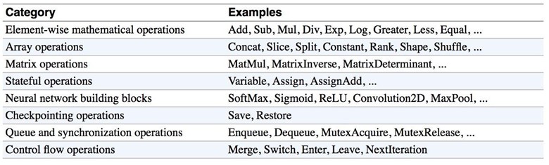
4. Data Types
Python Native Types
TensorFlow takes in Python native types such as Python boolean values, numeric values (integers, floats), and strings. Single values will be converted to 0-d tensors (or scalars), lists of values will be converted to 1-d tensors (vectors), lists of lists of values will be converted to 2-d
tensors (matrices), and so on. Example below is adapted from TensorFlow for Machine Intelligence.
|
t_0 = 19 # Treated as a 0-d tensor, or "scalar" tf.zeros_like(t_0) # ==> 0 tf.ones_like(t_0) # ==> 1 t_1 = [b"apple", b"peach", b"grape"] # treated as a 1-d tensor, or "vector" tf.zeros_like(t_1) # ==> [b'' b'' b''] tf.ones_like(t_1) # ==> TypeError t_2 = [[True, False, False], [False, False, True], [False, True, False]] # treated as a 2-d tensor, or "matrix" tf.zeros_like(t_2) # ==> 3x3 tensor, all elements are False tf.ones_like(t_2) # ==> 3x3 tensor, all elements are True |
TensorFlow Native Types
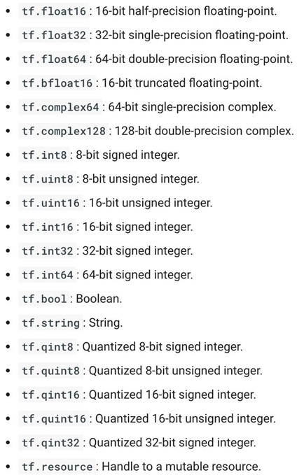
Like NumPy, TensorFlow also has its own data types as you've seen: tf.int32, tf.float32, together with more exciting types such as tf.bfloat, tf.complex, tf.quint. Below is the full list of TensorFlow data types, as literally screenshot from tf.DType class.
NumPy Data Types
By now, you've probably noticed the similarity between NumPy and TensorFlow. TensorFlow was designed to integrate seamlessly with Numpy, the package that has become the lingua franca of data science.
TensorFlow's data types are based on those of NumPy; in fact, np.int32 == tf.int32 returns True. You can pass NumPy types to TensorFlow ops.
|
tf.ones([2, 2], np.float32) ==> [[1.0 1.0], [1.0 1.0]] |
Remember our best friend tf.Session.run()? If the requested object is a Tensor, the output of will be a NumPy array.
TL;DR: Most of the times, you can use TensorFlow types and NumPy types interchangeably.
Note 1: There is a catch here for string data types. For numeric and boolean types, TensorFlow and NumPy dtypes match down the line. However, tf.string does not have an exact match in NumPy due to the way NumPy handles strings. TensorFlow can still import string arrays from NumPy perfectly fine -- just don't specify a dtype in NumPy!
Note 2: Both TensorFlow and NumPy are n-d array libraries. NumPy supports ndarray, but doesn't offer methods to create tensor functions and automatically compute derivatives, nor GPU support. There have been numerous efforts to create "NumPy for GPU", such as Numba, PyCUDA, gnumpy, but none has really taken off, so I guess TensorFlow is "NumPy for GPU". Please correct me if I'm wrong here.
Note 3: Using Python types to specify TensorFlow objects is quick and easy, and it is useful for prototyping ideas. However, there is an important pitfall in doing it this way. Python types lack the ability to explicitly state the data type, while TensorFlow's data types are more explicit. For example, all integers are the same type, but TensorFlow has 8-bit, 16-bit, 32-bit, and 64-bit integers available. Therefore, if you use a Python type, TensorFlow has to infer which data type you mean.
It's possible to convert the data into the appropriate type when you pass it into TensorFlow, but certain data types still may be difficult to declare correctly, such as complex numbers. Because of this, it is common to create hand-defined Tensor objects as NumPy arrays. However, always use TensorFlow types when possible.
5. Variables
Constants have been fun and now is the time to learn about what really matters: variables. The differences between a constant and a variable:
- A constant is, well, constant. Often, you'd want your weights and biases to be updated during training.
- A constant's value is stored in the graph and replicated wherever the graph is loaded. A variable is stored separately, and may live on a parameter server.
Point 2 means that constants are stored in the graph definition. When constants are memory expensive, such as a weight matrix with millions of entries, it will be slow each time you have to load the graph. To see what's stored in the graph's definition, simply print out the graph's protobuf. Protobuf stands for protocol buffer, "Google's language-neutral, platform-neutral, extensible mechanism for serializing structured data – think XML, but smaller, faster, and simpler."
|
import tensorflow as tf my_const = tf.constant([1.0, 2.0], name="my_const") print(tf.get_default_graph().as_graph_def()) |
Output:
|
node { name: "my_const" op: "Const" attr { key: "dtype" value { type: DT_FLOAT } } attr { key: "value" value { tensor { dtype: DT_FLOAT tensor_shape { dim { size: 2 } } tensor_content: "�00�00200?�00�00�00@" } } } } versions { producer: 24 } |
Creating variables
To declare a variable, you create an instance of the class tf.Variable. Note that it's written tf.constant with lowercase 'c' but tf.Variable with uppercase 'V'. It's because tf.constant is an op, while tf.Variable is a class with multiple ops.
|
x = tf.Variable(...) x.initializer # init x.value() # read op x.assign(...) # write op x.assign_add(...) # and more |
The old way to create a variable is simply call tf.Variable(<initial-value>, name=<optional-name>)
|
s = tf.Variable(2, name="scalar") m = tf.Variable([[0, 1], [2, 3]], name="matrix") W = tf.Variable(tf.zeros([784,10])) |
However, this old way is discouraged and TensorFlow recommends that we use the wrapper tf.get_variable, which allows for easy variable sharing. With tf.get_variable, we can provide variable's internal name, shape, type, and initializer to give the variable its initial value. Note that when we use tf.constant as an initializer, we don't need to provide shape.
|
tf.get_variable( name, shape=None, dtype=None, initializer=None, regularizer=None, trainable=True, collections=None, caching_device=None, partitioner=None, validate_shape=True, use_resource=None, custom_getter=None, constraint=None ) |
|
s = tf.get_variable("scalar", initializer=tf.constant(2)) m = tf.get_variable("matrix", initializer=tf.constant([[0, 1], [2, 3]])) W = tf.get_variable("big_matrix", shape=(784, 10), initializer=tf.zeros_initializer()) |
Initialize variables
You have to initialize a variable before using it. If you try to evaluate the variables before initializing them you'll run into FailedPreconditionError: Attempting to use uninitialized value. To get a list of uninitialized variables, you can just print them out:
|
print(session.run(tf.report_uninitialized_variables())) |
The easiest way is initialize all variables at once
|
with tf.Session() as sess: sess.run(tf.global_variables_initializer()) |
In this case, you use tf.Session.run() to fetch an initializer op, not a tensor op like we have used it previously.
To initialize only a subset of variables, you use tf.variables_initializer() with a list of variables you want to initialize:
|
with tf.Session() as sess: sess.run(tf.variables_initializer([a, b])) |
You can also initialize each variable separately using tf.Variable.initializer
|
with tf.Session() as sess: sess.run(W.initializer) |
Another way to initialize a variable is to load its value from a file. We will talk about it in a few weeks.
Evaluate values of variables
Similar to TensorFlow tensors, to get the value of a variable, we need to fetch it within a session.
|
# V is a 784 x 10 variable of random values V = tf.get_variable("normal_matrix", shape=(784, 10), initializer=tf.truncated_normal_initializer()) with tf.Session() as sess: sess.run(tf.global_variables_initializer()) print(sess.run(V)) |
You can also get a variable's value from tf.Variable.eval()
|
with tf.Session() as sess: sess.run(tf.global_variables_initializer()) print(V.eval()) |
Assign values to variables
We can assign a value to a variable using tf.Variable.assign()
|
W = tf.Variable(10) W.assign(100) with tf.Session() as sess: sess.run(W.initializer) print(W.eval()) # >> 10 |
Why 10 and not 100? W.assign(100) doesn't assign the value 100 to W, but instead create an assign op to do that. For this op to take effect, we have to run this op in session.
|
W = tf.Variable(10) assign_op = W.assign(100) with tf.Session() as sess: sess.run(assign_op) print(W.eval()) # >> 100 |
Note that we don't have to initialize W in this case, because assign() does it for us. In fact, the initializer op is an assign op that assigns the variable's initial value to the variable itself.
|
# in the source code self._initializer_op = state_ops.assign(self._variable, self._initial_value, validate_shape=validate_shape).op |
Interesting example:
|
# create a variable whose original value is 2 a = tf.get_variable('scalar', initializer=tf.constant(2)) a_times_two = a.assign(a * 2) with tf.Session() as sess: sess.run(tf.global_variables_initializer()) sess.run(a_times_two) # >> 4 sess.run(a_times_two) # >> 8 sess.run(a_times_two) # >> 16 |
For simple incrementing and decrementing of variables, TensorFlow includes the tf.Variable.assign_add() and tf.Variable.assign_sub() methods. Unlike tf.Variable.assign(), tf.Variable.assign_add() and tf.Variable.assign_sub() don't initialize your variables for you because these ops depend on the initial values of the variable.
|
W = tf.Variable(10) with tf.Session() as sess: sess.run(W.initializer) print(sess.run(W.assign_add(10))) # >> 20 print(sess.run(W.assign_sub(2))) # >> 18 |
Because TensorFlow sessions maintain values separately, each Session can have its own current value for a variable defined in a graph.
|
W = tf.Variable(10) sess1 = tf.Session() sess2 = tf.Session() sess1.run(W.initializer) sess2.run(W.initializer) print(sess1.run(W.assign_add(10))) # >> 20 print(sess2.run(W.assign_sub(2))) # >> 8 print(sess1.run(W.assign_add(100))) # >> 120 print(sess2.run(W.assign_sub(50))) # >> -42 sess1.close() sess2.close() |
When you have a variable that depends on another variable, suppose you want to declare U = W * 2
|
# W is a random 700 x 10 tensor W = tf.Variable(tf.truncated_normal([700, 10])) U = tf.Variable(W * 2) |
In this case, you should use initialized_value() to make sure that W is initialized before its value is used to initialize U.
|
U = tf.Variable(W.initialized_value() * 2) |
6. Interactive Session
You sometimes see InteractiveSession instead of Session. The only difference is an InteractiveSession makes itself the default session so you can call run() or eval() without explicitly call the session. This is convenient in interactive shells and IPython notebooks, as it avoids having to pass an explicit session object to run ops. However, it is complicated when you have multiple sessions to run.
|
sess = tf.InteractiveSession() a = tf.constant(5.0) b = tf.constant(6.0) c = a * b print(c.eval()) # we can use 'c.eval()' without explicitly stating a session sess.close() |
tf.get_default_session() returns the default session for the current thread. The returned Session will be the innermost session on which a Session or Session.as_default() context has been entered.
7. Control Dependencies
Sometimes, we have two or more independent ops and we'd like to specify which ops should be run first. In this case, we use tf.Graph.control_dependencies([control_inputs]).
|
# your graph g have 5 ops: a, b, c, d, e with g.control_dependencies([a, b, c]): # `d` and `e` will only run after `a`, `b`, and `c` have executed. d = ... e = … |
8. Importing Data
8.1 The old way: placeholders and feed_dict
Remember from the lecture 1 that a TensorFlow program often has 2 phases:
|
Phase 1: assemble a graph Phase 2: use a session to execute operations and evaluate variables in the graph |
We can assemble the graphs first without knowing the values needed for computation. This is equivalent to defining the function of x, y without knowing the values of x, y. For example:
are placeholders for the actual values.
With the graph assembled, we, or our clients, can later supply their own data when they need to execute the computation. To define a placeholder, we use:
|
tf.placeholder(dtype, shape=None, name=None) |
Dtype, shape, and name are self-explanatory. The only thing to note here is when you set the shape of the placeholder to None. shape=None means that tensors of any shape will be accepted. Using shape=None is easy to construct graphs, but nightmarish for debugging. You should always define the shape of your placeholders as detailed as possible. shape=None also breaks all following shape inference, which makes many ops not work because they expect certain rank.
|
a = tf.placeholder(tf.float32, shape=[3]) # a is placeholder for a vector of 3 elements b = tf.constant([5, 5, 5], tf.float32) c = a + b # use the placeholder as you would any tensor with tf.Session() as sess: print(sess.run(c)) |
When we try to get the value of c through a session, we will run into an error because to compute the value of c, we need to know the value of a. However, a is just a placeholder with no value. To supplement the value of placeholders, we use a feed_dict, which is basically a dictionary with keys being the placeholders, value being the values of those placeholders.
|
with tf.Session() as sess: # compute the value of c given the value of a is [1, 2, 3] print(sess.run(c, {a: [1, 2, 3]})) # [6. 7. 8.] |
Let's see how it looks in TensorBoard. Remember, first write the graph to the log file.
|
writer = tf.summary.FileWriter('graphs/placeholders',tf.get_default_graph()) |
and type the following in the terminal:
|
$ tensorboard --logdir='graphs/placeholders' |
As you can see, placeholder are treated like any other op. 3 is the shape of placeholder.

In the previous example, we feed one single value to the placeholder. What if we want to feed multiple data points to placeholder, for example, when we run computation through multiple data points in our training or testing set?
We can feed as many data points to the placeholder as we want by iterating through the data set and feed in the value one at a time.
|
with tf.Session() as sess: for a_value in list_of_a_values: print(sess.run(c, {a: a_value})) |
You can feed values to tensors that aren't placeholders. Any tensors that are feedable can be fed. To check if a tensor is feedable or not, use:
|
tf.Graph.is_feedable(tensor) |
|
a = tf.add(2, 5) b = tf.multiply(a, 3) with tf.Session() as sess: print(sess.run(b)) # >> 21 # compute the value of b given the value of a is 15 print(sess.run(b, feed_dict={a: 15})) # >> 45 |
feed_dict can be extremely useful to test your model. When you have a large graph and just want to test out certain parts, you can provide dummy values so TensorFlow won't waste time doing unnecessary computations.
8.2 The new way: tf.data
This is best to learn with examples, so we will cover it in the next lecture with linear and logistic regression.
9. The trap of lazy loading
One of the most common TensorFlow non-bug bugs I see is what my friend Danijar and I call "lazy loading". Lazy loading is a term that refers to a programming pattern when you defer declaring/initializing an object until it is loaded. In the context of TensorFlow, it means you defer creating an op until you need to compute it. For example, this is normal loading: you create the op z when you assemble the graph.
|
x = tf.Variable(10, name='x') y = tf.Variable(20, name='y') z = tf.add(x, y) with tf.Session() as sess: sess.run(tf.global_variables_initializer()) writer = tf.summary.FileWriter('graphs/normal_loading', sess.graph) for _ in range(10): sess.run(z) writer.close() |
This is what happens when someone decides to be clever and use lazy loading to save one line of code:
|
x = tf.Variable(10, name='x') y = tf.Variable(20, name='y') with tf.Session() as sess: sess.run(tf.global_variables_initializer()) writer = tf.summary.FileWriter('graphs/lazy_loading', sess.graph) for _ in range(10): sess.run(tf.add(x, y)) print(tf.get_default_graph().as_graph_def()) writer.close() |
Let's see the graphs for them on TensorBoard. Note that you can open Tensorboard with logdir='graphs' and you can easily switch between normal_loading graph and lazy_loading graph.
They seem ostensibly similar. The first graph is normal loading, and the second is lazy loading.
Let's look at the graph definition. Remember that to print out the graph definition, we use:
|
print(tf.get_default_graph().as_graph_def()) |
The protobuf for the graph in normal loading has only 1 node "Add":
|
node { name: "Add" op: "Add" input: "x/read" input: "y/read" attr { key: "T" value { type: DT_INT32 } } } |
On the other hand, the protobuf for the graph in lazy loading has 10 copies of the node "Add". It adds a new node "Add" every time you want to compute z!
|
node { name: "Add_1" op: "Add" input: "x_1/read" input: "y_1/read" attr { key: "T" value { type: DT_INT32 } } } … … … node { name: "Add_10" op: "Add" ... } |
You probably think: "This is stupid. Why would I want to compute the same value more than once?" and think that it's a bug that nobody will ever commit. It happens more often than you think. For example, you might want to compute the same loss function or make the same prediction every batch of training samples. If you aren't careful, you can add thousands of unnecessary nodes to your graph. Your graph definition becomes bloated, slow to load and expensive to pass around.
There are two ways to avoid this bug. First, always separate the definition of ops and their execution when you can. But when it is not possible because you want to group related ops into classes, you can use Python @property to ensure that your function is only loaded once when it's first called. This is not a Python course so I won't dig into how to do it. But if you want to know, check out this wonderful blog post by Danijar Hafner.