Lecture note 5: word2vec + manage experiments
Word2vec
Most of you are probably already familiar with word embedding and understand the importance of a model like word2vec. For those who aren't, Stanford CS 224N's lecture on word vectors is a great resource. When you're at it, it might be a good idea to check out the following two papers:
Distributed Representations of Words and Phrases and their Compositionality (Mikolov et al., 2013)
Efficient Estimation of Word Representations in Vector Space (Mikolov et al., 2013)
At a high level, we need to find an efficient way to represent textual data (in this case, words) so that we can use this representation to solve natural language tasks. Word embeddings form the backbone in the solutions to many tasks such as language modeling, machine translation, sentiment analysis, etc.
Created by a team of researchers led by Tomas Mikolov, word2vec is a group of models that are used to produce word embeddings. There are two main models used in word2vec: skip-gram and CBOW.
|
Skip-gram vs CBOW (Continuous Bag-of-Words) Algorithmically, these models are similar, except that CBOW predicts center words from context words, while the skip-gram does the inverse and predicts source context-words from the center words. For example, if we have the sentence: ""The quick brown fox jumps"", then CBOW tries to predict ""brown"" from ""the"", ""quick"", ""fox"", and ""jumps"", while skip-gram tries to predict ""the"", ""quick"", ""fox"", and ""jumps"" from ""brown"". Statistically it has the effect that CBOW smoothes over a lot of the distributional information (by treating an entire context as one observation). For the most part, this turns out to be a useful thing for smaller datasets. However, skip-gram treats each context-target pair as a new observation, and this tends to do better when we have larger datasets. |
In this lecture, we will build word2vec, the skip-gram model. In this model, to get the vector representations of words, we train a simple neural network with a single hidden layer to perform a certain task, but then we don't use that neural network for the task we train it on. Instead, we care about the weights of the hidden layer. These weights are actually the "word vectors", or "embedding matrix" that we're trying to learn.
The certain, fake task we're going to train our model on is predicting the neighboring (context) words given the center word. Given a specific word in a sentence (the center word), look at the words nearby and pick one at random. The network is going to tell us the probability for every word in our vocabulary of being a neighbor to a specific word. Chris McCormick wrote a tutorial that explains the skip-gram model wonderfully if you want more details.
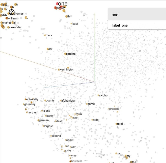
Vector representations of words visualized with t-SNE projected on a 3D space, using TensorBoard.
Softmax, Negative Sampling, and Noise Contrastive Estimation
To get the distribution of the possible neighboring words, in theory, we often use softmax. Softmax maps arbitrary values to a probability distribution . In this case, is the probability that is a neighboring word of a specific word we are considering.
However, the normalization term in the denominator requires us to perform exp on all words in the dictionary and sum the results up, which could be millions of words. Even if you disregard uncommon words, a natural language model doesn't perform well unless you consider at least tens of thousands of the most common words. The normalization term causes softmax to be computationally prohibitive.
There are two main approaches to circumvent this bottleneck: hierarchical softmax and sample-based softmax. Mikolov et al. have shown in their paper Distributed Representations of Words and Phrases and their Compositionality that for training the skip-gram model, negative sample results in faster training and better vector representations for frequent words, compared to more complex hierarchical softmax.
Negative sampling, as the name suggests, belongs to the family of sample-based approaches. This family also includes importance sampling and target sampling. Negative sampling is actually a simplified model of an approach called Noise Contrastive Estimation (NCE), e.g. negative sampling makes certain assumption about the number of noise samples to generate -- let's call it -- and the distribution of noise samples -- let's call it -- such that to simplify computation. For more details, please see Sebastian Rudder's On word embeddings - Part 2: Approximating the Softmax and Chris Dyer's Notes on Noise Contrastive Estimation and Negative Sampling.
While negative sampling is useful for the learning word embeddings, it doesn't have the theoretical guarantee that its derivative tends towards the gradient of the softmax function. NCE, on the contrary, offers this guarantee as the number of noise samples increases. Mnih and Teh (2012) reported that 25 noise samples are sufficient to match the performance of the regular softmax, with an expected speed-up factor of about 45. For this reason, in this example, we will be using NCE.
Note that sample-based approaches, whether it's negative sampling or NCE, are only useful at training time -- during inference, the full softmax still needs to be computed to obtain a normalized probability.
Dataset
text8 is the first 100 MB of cleaned text of the English Wikipedia dump on Mar. 3, 2006 (whose link is no longer available). We use text that has already been pre-processed because it takes a lot of time to process the raw text and we'd rather use the time in this class to focus on TensorFlow. We can download the dataset here. The file word_utils.py on our GitHub repo has a script to download and read the text
100MB is not enough to train really good word embeddings, but enough to see some interesting relations. There are 17,005,207 tokens if you count tokens by splitting the text by blank space. For better results, you should use the dataset fil9 of the first bytes of the Wikipedia dump, as described on Matt Mahoney's website.
Implementing word2vec
In this example, we implement skip-gram without eager execution. For example with eager execution, please see examples/04_word2vec_eager.py. If you want to give it a try first, use examples/04_word2vec_eager_starter.py.
Phase 1: Assemble the graph
1. Create dataset and generate samples from them
Input is the center word and output is the neighboring (context) word. Instead of feeding words into our model, we create a dictionary of the most common words, and feed the indices of those words. For example, if the center word is the word in the vocabulary, we input the number 999.
Each sample input is a scalar, so BATCH_SIZE of sample inputs have shape [BATCH_SIZE] Similarly, BATCH_SIZE of sample outputs have shape [BATCH_SIZE, 1].
|
dataset = tf.data.Dataset.from_generator(gen, (tf.int32, tf.int32), (tf.TensorShape([BATCH_SIZE]), tf.TensorShape([BATCH_SIZE, 1]))) iterator = dataset.make_initializable_iterator() center_words, target_words = iterator.get_next() |
2. Define the weight (in this case, embedding matrix)
Each row corresponds to the representation vector of one word. If one word is represented with a vector of size EMBED_SIZE, then the embedding matrix will have shape [VOCAB_SIZE, EMBED_SIZE]. We initialize the embedding matrix to value from a random distribution. In this case, let's choose uniform distribution.
|
embed_matrix = tf.get_variable('embed_matrix', shape=[VOCAB_SIZE, EMBED_SIZE], initializer=tf.random_uniform_initializer()) |
3. Inference (compute the forward path of the graph)
Our goal is to get the vector representations of words in our dictionary. Remember that the embed_matrix has dimension VOCAB_SIZE x EMBED_SIZE, with each row of the embedding matrix corresponds to the vector representation of the word at that index. So to get the representation of all the center words in the batch, we get the slice of all corresponding rows in the embedding matrix. TensorFlow provides a convenient method to do so.
|
tf.nn.embedding_lookup( params, ids, partition_strategy='mod', name=None, validate_indices=True, max_norm=None ) |
This method is really useful when it comes to matrix multiplication with one-hot vectors because it saves us from doing a bunch of unnecessary computation that will return 0 anyway. An illustration from Chris McCormick for multiplication of a one-hot vector with a matrix.
So, to get the embedding (or vector representation) of the input center words, we use this:
|
embed = tf.nn.embedding_lookup(embed_matrix, center_words, name='embed') |
4. Define the loss function
While NCE is cumbersome to implement in pure Python, TensorFlow already implemented it for us.
|
tf.nn.nce_loss( weights, biases, labels, inputs, num_sampled, num_classes, num_true=1, sampled_values=None, remove_accidental_hits=False, partition_strategy='mod', name='nce_loss' ) |
Note that by the way the function is implemented, the third argument is actually inputs, and the fourth is labels. This ambiguity can be quite troubling sometimes, but keep in mind that TensorFlow is still new and growing and therefore might not be perfect. Nce_loss source code can be found here.
For nce_loss, we need weights and biases for the hidden layer to calculate NCE loss. They will be updated by optimizer during training. After sampling, the final output score will be computed as followed. This computation is done internally in tf.nn.nce_loss operation.
|
tf.matmul(embed, tf.transpose(nce_weight)) + nce_bias |
|
nce_weight = tf.get_variable('nce_weight', |
Then we define loss:
|
loss = tf.reduce_mean(tf.nn.nce_loss(weights=nce_weight, biases=nce_bias, labels=target_words, inputs=embed, num_sampled=NUM_SAMPLED, num_classes=VOCAB_SIZE)) |
5. Define optimizer
We will use the good old gradient descent.
|
optimizer = tf.train.GradientDescentOptimizer(LEARNING_RATE).minimize(loss) |
Phase 2: Execute the computation
We will create a good old session to run the optimizer to minimize the loss, and report the loss value back to us. Don't forget to reinitialize your iterator!
|
with tf.Session() as sess: sess.run(iterator.initializer) sess.run(tf.global_variables_initializer())
writer = tf.summary.FileWriter('graphs/word2vec_simple', sess.graph)
for index in range(NUM_TRAIN_STEPS): try: loss_batch, _ = sess.run([loss, optimizer]) except tf.errors.OutOfRangeError: sess.run(iterator.initializer) writer.close() |
You can see the full basic model on the class's GitHub repo under the name word2vec.py.
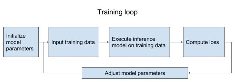
Interface: How to structure your TensorFlow model
All models we've built so far have more or less have the same structure:
Phase 1: assemble your graph
1. Import data (either with tf.data or with placeholders)
2. Define the weights
3. Define the inference model
4. Define loss function
5. Define optimizer
Phase 2: execute the computation
Which is basically training your model. There are a few steps:
1. Initialize all model variables for the first time.
2. Initialize iterator / feed in the training data.
3. Execute the inference model on the training data, so it calculates for each training input example the output with the current model parameters.
4. Compute the cost
5. Adjust the model parameters to minimize/maximize the cost depending on the model.
Here is a visualization of training loop from the book TensorFlow for Machine Intelligence (Abrahams et al., 2016).
It took us about 20 lines of code to build a word embedding model! It's fast but … "what happened to decomposition?" After we've spent an ungodly amount of time building a model, we'd like to use it more than once.
Question: how do we make our model most easy to reuse?
Hint: take advantage of Python's object-oriented-ness.
Answer: build our model as a class!
Our model base class should follow the interface. We combined step 3 and 4 because we want to put embed under the name scope of "NCE loss".
|
class SkipGramModel: """ Build the graph for word2vec model """ def __init__(self, params): pass
def _import_data(self): """ Step 1: import data """ pass
def _create_embedding(self): """ Step 2: in word2vec, it's actually the weights that we care about """ pass
def _create_loss(self): """ Step 3 + 4: define the inference + the loss function """ pass
def _create_optimizer(self): """ Step 5: define optimizer """ pass |
Visualize embeddings
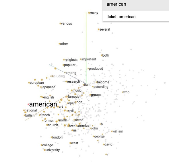
Now let's see what our model finds after training it for 100,000 iterations. If we visualize our embedding with t-SNE, we will see something like this.

It's hard to see in 2D, but we'll see in class in 3D that all the number (one, two, …, zero) are grouped in a line on the bottom right, next to all the alphabet (a, b, …, z) and names (john, james, david, and such). All the months are grouped together. "Do", "does", "did" are also grouped together and so on.
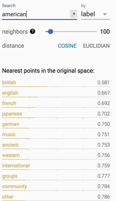
If you print out the closest words to 'american', you will find its closest cosine neighbors are 'british' and 'english'. Fair enough.
How about words closest to 'government'?

|
t-SNE (from Wikipedia)
t-distributed stochastic neighbor embedding (t-SNE) is a machine learning algorithm for dimensionality reduction developed by Geoffrey Hinton and Laurens van der Maaten. It is a nonlinear dimensionality reduction technique that is particularly well-suited for embedding high-dimensional data into a space of two or three dimensions, which can then be visualized in a scatter plot. Specifically, it models each high-dimensional object by a two- or three-dimensional point in such a way that similar objects are modeled by nearby points and dissimilar objects are modeled by distant points.
The t-SNE algorithm comprises two main stages. First, t-SNE constructs a probability distribution over pairs of high-dimensional objects in such a way that similar objects have a high probability of being picked, whilst dissimilar points have an extremely small probability of being picked. Second, t-SNE defines a similar probability distribution over the points in the low-dimensional map, and it minimizes the Kullback–Leibler divergence between the two distributions with respect to the locations of the points in the map. Note that whilst the original algorithm uses the Euclidean distance between objects as the base of its similarity metric, this should be changed as appropriate. |
If you haven't used t-SNE, you should start using it! It's super cool.
You can visualize more than word embeddings, aka, you can visualize any vector representations of anything! Have you read Chris Olah's blog post about visualizing MNIST? t-SNE made MNIST desirable! Image below is from Olah's blog.

We can also visualize our embeddings using PCA too.
And we did all that visualization with less than 10 lines of code using TensorFlow projector with TensorBoard! The tool is super useful, albeit a bit finicky to use. The visualization will be stored in visualization folder. To see it, run "'tensorboard --logdir='visualization'".
|
from tensorflow.contrib.tensorboard.plugins import projector
def visualize(self, visual_fld, num_visualize): # create the list of num_variable most common words to visualize word2vec_utils.most_common_words(visual_fld, num_visualize)
saver = tf.train.Saver() with tf.Session() as sess: sess.run(tf.global_variables_initializer()) ckpt = tf.train.get_checkpoint_state(os.path.dirname('checkpoints/checkpoint'))
# if that checkpoint exists, restore from checkpoint if ckpt and ckpt.model_checkpoint_path: saver.restore(sess, ckpt.model_checkpoint_path)
final_embed_matrix = sess.run(self.embed_matrix)
# you have to store embeddings in a new variable embedding_var = tf.Variable(final_embed_matrix[:num_visualize], name='embeded') sess.run(embedding_var.initializer)
config = projector.ProjectorConfig() summary_writer = tf.summary.FileWriter(visual_fld)
# add embedding to the config file embedding = config.embeddings.add() embedding.tensor_name = embedding_var.name
# link this tensor to the file with the first NUM_VISUALIZE words of vocab embedding.metadata_path = os.path.join(visual_fld,[file_of_most_common_words])
# saves a configuration file that TensorBoard will read during startup. projector.visualize_embeddings(summary_writer, config) saver_embed = tf.train.Saver([embedding_var]) saver_embed.save(sess, os.path.join(visual_fld, 'model.ckpt'), 1) |
To see the full code, please see examples/04_word2vec_visualize.py on the class's GitHub repo.
Variable sharing
Name scope
Let's give the tensors name and see how our word2vec model looks like on TensorBoard.
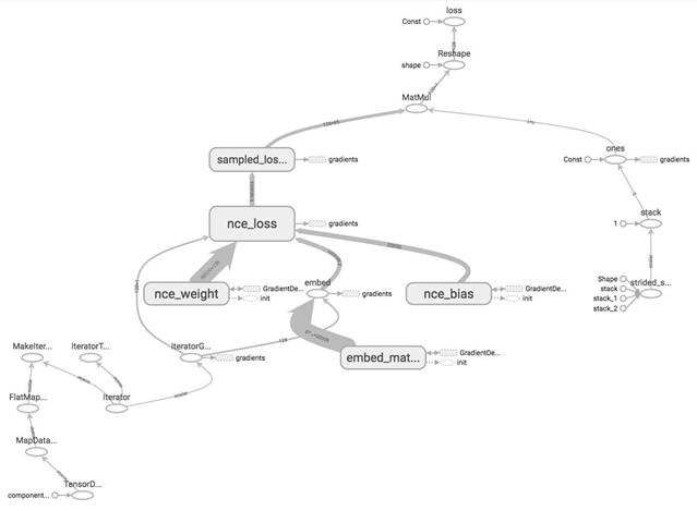
As you can see in the graph, the nodes are scattering all over, rendering the graph difficult to read. TensorBoard doesn't know which nodes are similar to which nodes and should be grouped together. This can make debugging your graph daunting when you build complex models with hundreds of ops.
How can we let TensorBoard know which nodes should be grouped together? For example, we would like to group all ops related to input/output together, and group all ops related to NCE loss together. TensorFlow lets us do that with name_scope. You can put all the ops that you want to group together under the block:
|
with tf.name_scope(name_of_that_scope): # declare op_1 # declare op_2 # ... |
For example, our graph can have four name scopes: "data", "embed", "loss", and "optimizer".
|
with tf.name_scope('data'): iterator = dataset.make_initializable_iterator() center_words, target_words = iterator.get_next()
with tf.name_scope('embed'): embed_matrix = tf.get_variable('embed_matrix', shape=[VOCAB_SIZE, EMBED_SIZE], initializer=tf.random_uniform_initializer()) embed = tf.nn.embedding_lookup(embed_matrix, center_words, name='embedding')
with tf.name_scope('loss'): nce_weight = tf.get_variable('nce_weight', shape=[VOCAB_SIZE, EMBED_SIZE], initializer=tf.truncated_normal_initializer()) nce_bias = tf.get_variable('nce_bias', initializer=tf.zeros([VOCAB_SIZE]))
loss = tf.reduce_mean(tf.nn.nce_loss(weights=nce_weight, biases=nce_bias, labels=target_words, inputs=embed, num_sampled=NUM_SAMPLED, num_classes=VOCAB_SIZE), name='loss')
with tf.name_scope('optimizer'): optimizer = tf.train.GradientDescentOptimizer(LEARNING_RATE).minimize(loss) |
When you visualize that on TensorBoard, you will see your nodes are grouped into neat blocks.

You can click on the plus sign on top of each name scope block to see all the ops inside that block. Take your time to play around with it.
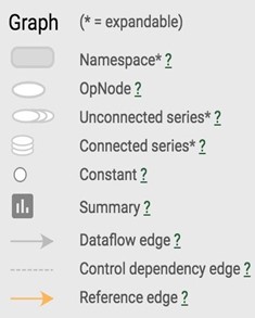
TensorBoard has three kinds of edges: the solid grey arrows, the solid orange arrows, and the dotted arrows. The solid grey arrows represent data flow edges. For example, the op tf.add(x + y) get the values from x and y. The solid orange arrows are reference edges which represent which ops can mutate which ops. In this graph, it means that our optimizer can mutate -- in this case, update through backprop -- nce_weights, nce_bias, and embed_matrix.The dotted arrows represent control dependence edges. For example, nce_weight can only be executed after init -- a variable can only be used after being initialized. Control dependencies can be declared using tf.Graph.control_dependencies(control_inputs).
To see the full model of word2vec with name scope defined, see examples/04_word2vec_visualize.py on the class's GitHub repo.
Variable scope
One of the questions I'm often asked is: "So what's the difference between name_scope and variable_scope". While both create namespaces, the main thing variable_scope does is to facilitate variable sharing. Let's explore why we need variable sharing.
Assume that we want to create a neural network with two hidden layers as followed. We then called that two hidden layers network on two different input x1 and x2.
|
x1 = tf.truncated_normal([200, 100], name='x1') x2 = tf.truncated_normal([200, 100], name='x2') |
|
def two_hidden_layers(x): assert x.shape.as_list() == [200, 100] w1 = tf.Variable(tf.random_normal([100, 50]), name="h1_weights") b1 = tf.Variable(tf.zeros([50]), name="h1_biases") h1 = tf.matmul(x, w1) + b1 assert h1.shape.as_list() == [200, 50] w2 = tf.Variable(tf.random_normal([50, 10]), name="h2_weights") b2 = tf.Variable(tf.zeros([10]), name="h2_biases") logits = tf.matmul(h1, w2) + b2 return logits
logits1 = two_hidden_layers(x1) logits2 = two_hidden_layers(x2) |
If we visualize this on TensorBoard, this is what we see.
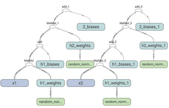
Each time you call two network, TensorFlow creates a different set of variables, while in fact, you want the network to share the same variables for all inputs, whether it's x1, x2, or more. To do this, we first need to use tf.get_variable(). When we create a variable with tf.get_variable(), it first checks whether that variable exists. If it does, reuse it. If not, create a new one. However, if we simply replace tf.Variable() with tf.get_variable() such as the following:
|
def two_hidden_layers_2(x): assert x.shape.as_list() == [200, 100] w1 = tf.get_variable("h1_weights", [100, 50], initializer=tf.random_normal_initializer()) b1 = tf.get_variable("h1_biases", [50], initializer=tf.constant_initializer(0.0)) h1 = tf.matmul(x, w1) + b1 assert h1.shape.as_list() == [200, 50] w2 = tf.get_variable("h2_weights", [50, 10], initializer=tf.random_normal_initializer()) b2 = tf.get_variable("h2_biases", [10], initializer=tf.constant_initializer(0.0)) logits = tf.matmul(h1, w2) + b2 return logits |
We will run into this error:
|
ValueError: Variable h1_weights already exists, disallowed. Did you mean to set reuse=True or reuse=tf.AUTO_REUSE in VarScope? |
To avoid this, we need to put all variables we want to use in a VarScope, and set that VarScope to be reusable.
|
with tf.variable_scope('two_layers') as scope: logits1 = two_hidden_layers_2(x1) scope.reuse_variables() logits2 = two_hidden_layers_2(x2) def fully_connected(x, output_dim, scope): with tf.variable_scope(scope) as scope: w = tf.get_variable("weights", [x.shape[1], output_dim], initializer=tf.random_normal_initializer()) b = tf.get_variable("biases", [output_dim], initializer=tf.constant_initializer(0.0)) return tf.matmul(x, w) + b
def two_hidden_layers(x): h1 = fully_connected(x, 50, 'h1') h2 = fully_connected(h1, 10, 'h2')
with tf.variable_scope('two_layers') as scope: logits1 = two_hidden_layers(x1) scope.reuse_variables() logits2 = two_hidden_layers(x2) |
Let's look at TensorBoard.

There's only one set of variables now, all within the variable_scope two_layers. They take in two different inputs x1 and x2. tf.variable_scope("name") implicitly opens a tf.name_scope("name").
In our code, we write code for each layer. When we have more layers that are similar in structure, we probably want to make our code more reusable.
|
def fully_connected(x, output_dim, scope): with tf.variable_scope(scope) as scope: w = tf.get_variable('weights', [x.shape[1], output_dim], initializer=tf.random_normal_initializer()) b = tf.get_variable('biases', [output_dim], initializer=tf.constant_initializer(0.0)) return tf.matmul(x, w) + b
def two_hidden_layers(x): h1 = fully_connected(x, 50, 'h1') h2 = fully_connected(h1, 10, 'h2')
with tf.variable_scope('two_layers') as scope: logits1 = two_hidden_layers(x1) scope.reuse_variables() logits2 = two_hidden_layers(x2) |
You can scale it to infinitely many layers with many different kinds of activation functions!
Graph collections
As you create a model, you might put your variables to different parts of the graph. Sometimes, you'd want an easy way to access them. tf.get_collection lets you access a certain collection of variables, with key being the name of the collection, scope is the scope of the variables.
|
tf.get_collection( key, scope=None ) |
By default, all variables are placed in tf.GraphKeys.GLOBAL_VARIABLES. To get all variables in scope "my_scope", simply call. This turns a list of variables in "my_scope".
|
tf.get_collection(tf.GraphKeys.GLOBAL_VARIABLES, scope='my_scope') |
If you set trainable=True (which is always set by default) when you create your variable, that variable will be in the collection tf.GraphKeys.TRAINABLE_VARIABLES.
You can have collections of ops that aren't variables. And yes, you can create your own collections with tf.add_to_collection(name, value). For example, you can create a collection of initializers and add all init ops to that.
The standard library uses various well-known names to collect and retrieve values associated with a graph. For example, the tf.train.Optimizer subclasses default to optimizing the variables collected under tf.GraphKeys.TRAINABLE_VARIABLES if none is specified, but it is also possible to pass an explicit list of variables. For the list of predefined graph keys, please see the official documentation.
Manage experiments
We've built a word2vec model and it seems to be working pretty well using such a small dataset. We know that it'd take much longer time for a larger dataset, and we also know that training more complicated models can take an ungodly amount of time. For example, a machine translation models can take up to days, if not months on a single GPU. Many computer vision and reinforcement learning tasks require a really long time and a lot of patience.
It's difficult to let our models run for days, wait and then make adjustment. If the computer or the cluster crashes, the training is interrupted and we'll have to run our model all over again! It's crucial to be able to stop training at any point, for any reason, and resume training as if nothing happens. It will be helpful for analyzing our models, as this allows us closely inspect our models after any number of training steps.
Another problem that researchers often face is how to replicate research results. When building and training neural networks, we often use randomization. For example, we randomize the weights for our models, or we shuffle the order of our training samples. It's important to learn how to control this random factor in our models.
In this part of the lecture, we will go over the excellent set of tools that TensorFlow provides to help us manage our experiments, including but not limited to tf.train.Saver() class, TensorFlow's random state, and visualization our training progress (aka more TensorBoard).
tf.train.Saver()
A good practice is to periodically save the model's parameters after a certain number of steps or epochs so that we can restore/retrain our model from that step if need be. The tf.train.Saver() class allows us to do so by saving the graph's variables in binary files.
|
tf.train.Saver.save( sess, save_path, global_step=None, latest_filename=None, meta_graph_suffix='meta', write_meta_graph=True, write_state=True ) |
For example, if we want to save the variables of the graph after every 1000 training steps, we do the following:
|
# define model
# create a saver object saver = tf.train.Saver()
# launch a session to execute the computation with tf.Session() as sess: # actual training loop for step in range(training_steps): sess.run([optimizer]) if (step + 1) % 1000 == 0: saver.save(sess, 'checkpoint_directory/model_name', global_step=global_step) |
In TensorFlow lingo, the step at which you save your graph's variables is called a checkpoint. Since we will be creating many checkpoints, it's helpful to append the number of training steps our model has gone through a variable called global_step. It's a variable you'd see in many TensorFlow programs. We first need to create it, initialize it to 0 and set it to be not trainable, since we don't want TensorFlow to optimize it.
|
global_step = tf.Variable(0, dtype=tf.int32, trainable=False, name='global_step') |
We need to pass global_step as a parameter to the optimizer so it knows to increment global_step by one with each training step.
|
optimizer = tf.train.GradientDescentOptimizer(lr).minimize(loss,global_step=global_step) |
To save the current values of variables in the folder 'checkpoints', we use this:
|
saver.save(sess, 'checkpoints/model-name', global_step=global_step) |
To restore the variables, we use tf.train.Saver.restore(sess, save_path). For example, to restore the checkpoint at the step.
|
saver.restore(sess, 'checkpoints/skip-gram-10000') |
But of course, we can only load saved variables if there is a valid checkpoint. What you probably want to do is that if there is a checkpoint, restore it. If there isn't, train from the start. TensorFlow allows you to get checkpoint from a directory with tf.train.get_checkpoint_state('directory-name'). The code for checking looks something like this:
|
ckpt = tf.train.get_checkpoint_state(os.path.dirname('checkpoints/checkpoint')) if ckpt and ckpt.model_checkpoint_path: saver.restore(sess, ckpt.model_checkpoint_path) |
The file checkpoint automatically keeps track of the path to the latest checkpoint, so if we find the latest checkpoint from , 'checkpoints/checkpoint' we can always get the latest checkpoint. This is an example of what the file 'checkpoints/checkpoint' looks like.
|
model_checkpoint_path: "skip-gram-21999" all_model_checkpoint_paths: "skip-gram-13999" all_model_checkpoint_paths: "skip-gram-15999" all_model_checkpoint_paths: "skip-gram-17999" all_model_checkpoint_paths: "skip-gram-19999" all_model_checkpoint_paths: "skip-gram-21999" |
So our training loop for word2vec now looks like this:
|
saver = tf.train.Saver()
initial_step = 0 utils.safe_mkdir('checkpoints')
with tf.Session() as sess: sess.run(self.iterator.initializer) sess.run(tf.global_variables_initializer())
# if a checkpoint exists, restore from the latest checkpoint ckpt = tf.train.get_checkpoint_state(os.path.dirname('checkpoints/checkpoint')) if ckpt and ckpt.model_checkpoint_path: saver.restore(sess, ckpt.model_checkpoint_path)
writer = tf.summary.FileWriter('graphs/word2vec' + str(self.lr), sess.graph)
for index in range(num_train_steps): try: sess.run(self.optimizer) # save the model every 1000 steps if (index + 1) % 1000 == 0: saver.save(sess, 'checkpoints/skip-gram', index) except tf.errors.OutOfRangeError: sess.run(self.iterator.initializer)
writer.close() |
If you go to the folder 'checkpoints', you will see files like the below:

By default, saver.save() stores all variables of the graph, and this is recommended. However, you can also choose what variables to store by passing them in as a list or a dict when we create the saver object. This is an example from TensorFlow official documentation.
|
v1 = tf.Variable(..., name='v1') v2 = tf.Variable(..., name='v2')
# pass the variables as a dict: saver = tf.train.Saver({'v1': v1, 'v2': v2})
# pass them as a list saver = tf.train.Saver([v1, v2])
# passing a list is equivalent to passing a dict with the variable op names # as keys saver = tf.train.Saver({v.op.name: v for v in [v1, v2]}) |
Note that savers only save variables, not the entire graph, so we still have to create the graph ourselves, and then load in variables. The checkpoints specify the way to map from variable names to tensors.
What people usually do is not just save the parameters from the last iteration, but also save the parameters that give the best result so far so that you can evaluate your model on the best parameters so far.
tf.summary
We've been using matplotlib to visualize our losses and accuracy, which is unnecessary because TensorBoard provides us with a great set of tools to visualize our summary statistics during our training. Some popular statistics to visualize is loss, average loss, accuracy. You can visualize them as scalar plots, histograms, or even images. So we have a new namescope in our graph to hold all the summary ops.
|
def _create_summaries(self): with tf.name_scope("summaries"): tf.summary.scalar("loss", self.loss) tf.summary.scalar("accuracy", self.accuracy) tf.summary.histogram("histogram loss", self.loss) # because you have several summaries, we should merge them all # into one op to make it easier to manage self.summary_op = tf.summary.merge_all() |
Because it's an op, you have to execute it with sess.run()
|
loss_batch, _, summary = sess.run([model.loss, model.optimizer, model.summary_op], feed_dict=feed_dict) |
Now you've obtained the summary, you need to write the summary to file using the same FileWriter object we created to visualize our graph.
|
writer.add_summary(summary, global_step=step) |
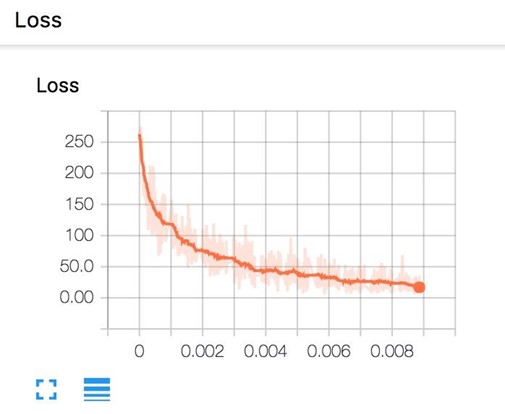
Now, if you go run tensorboard and go to http://localhost:6006/, in the Scalars page, you will see the plot of your scalar summaries. This is the summary of your loss in scalar plot.
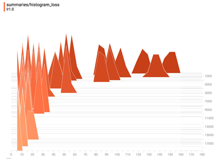
And the loss in histogram plot.
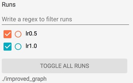
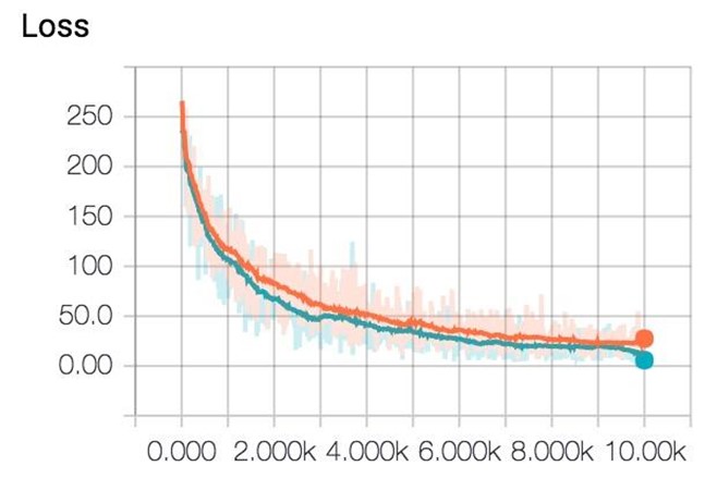
If you save your summaries into different sub-folder in your graph folder, you can compare your progresses. For example, the first time we run our model with learning rate 1.0, we save it in 'improved_graph/lr1.0' and the second time we run our model, we save it in 'improved_graph/lr0.5', on the left corner of the Scalars page, we can toggle the plots of these two runs to compare them. This can be really helpful when you want to compare the progress made with different optimizers or different parameters.
You can write a Python script to automate the naming of folders where you store the graphs/plots of each experiment.
You can visualize the statistics as images using tf.summary.image.
|
tf.summary.image(name, tensor, max_outputs=3, collections=None) |
Control randomization
I never realized what an oxymoron "control randomization" sounds like until I've written it down, but the truth is that you often have to control the randomization process to get stable results for your experiments. You're probably familiar with random seed and random state from NumPy. TensorFlow doesn't allow you to get random state the way NumPy does (at least not that I know of -- I will double check), but it does allow you to get stable results in randomization through two ways:
1. Set random seed at operation level. All random tensors allow you to pass in seed value in their initialization. For example:
|
my_var = tf.Variable(tf.truncated_normal((-1.0,1.0), stddev=0.1, seed=0)) |
Note that, session is the thing that keeps track of random state, so each new session will start the random state all over again.
|
c = tf.random_uniform([], -10, 10, seed=2)
with tf.Session() as sess: print sess.run(c) # >> 3.57493 print sess.run(c) # >> -5.97319 |
|
c = tf.random_uniform([], -10, 10, seed=2)
with tf.Session() as sess: print sess.run(c) # >> 3.57493
with tf.Session() as sess: print sess.run(c) # >> 3.57493 |
With operation level random seed, each op keeps its own seed.
|
c = tf.random_uniform([], -10, 10, seed=2) d = tf.random_uniform([], -10, 10, seed=2)
with tf.Session() as sess: print sess.run(c) # >> 3.57493 print sess.run(d) # >> 3.57493 |
2. Set random seed at graph level with tf.Graph.seed
|
tf.set_random_seed(seed) |
If you don't care about the randomization for each op inside the graph, but just want to be able to replicate result on another graph (so that other people can replicate your results on their own graph), you can use tf.set_random_seed instead. Setting the current TensorFlow random seed affects the current default graph only.
For example, you have two models a.py and b.py that have identical code:
|
import tensorflow as tf
tf.set_random_seed(2) c = tf.random_uniform([], -10, 10) d = tf.random_uniform([], -10, 10)
with tf.Session() as sess: print sess.run(c) print sess.run(d) |
Without graph level seed, running python a.py and b.py will return 2 completely different results, but with tf.set_random_seed, you will get two identical results:
|
$ python a.py >> -4.00752 >> -2.98339
$ python b.py >> -4.00752 >> -2.98339 |
Autodiff (how TensorFlow takes gradients)
In all the models we've built so far, we haven't taken a single gradient. All we need to do is to build a forward pass and TensorFlow takes care of the backward path for us. For example, if tensor C depends on a set of previous nodes, the gradient of C with respect to those previous nodes can be automatically computed with a built-in function, even if there are many layers in between them.
TensorFlow uses what's known as the reverse mode automatic differentiation. It allows you to take derivative of a function at roughly the same cost as computing the original function. Gradients are computed by creating additional nodes and edges in the graph. For example, you need to compute the gradients of C with respect to I, first TensorFlow looks for the path between these two nodes. Once the path is found, TensorFlow starts at C and moves backward toward I. For every operation on this backward path, a node is added to the graph, composing the partial gradients of each added node via the chain rule. This process is visualized in TensorFlow white paper:

To compute partial gradients, we can use tf.gradients()
|
tf.gradients(ys, xs, grad_ys=None, name='gradients', colocate_gradients_with_ops=False, gate_gradients=False, aggregation_method=None) |
tf.gradients(ys, [xs]) with [xs] stands for a list of tensors with respect to those you're trying to compute the gradient of ys. It will return a list of gradient values.
|
x = tf.Variable(2.0) y = 2.0 * (x ** 3)
grad_y = tf.gradients(y, x) with tf.Session() as sess: sess.run(x.initializer) print sess.run(grad_y) # >> 24.0 |
|
x = tf.Variable(2.0) y = 2.0 * (x ** 3) z = 3.0 + y ** 2
grad_z = tf.gradients(z, [x, y]) with tf.Session() as sess: sess.run(x.initializer) print sess.run(grad_z) # >> [768.0, 32.0] # 768 is the gradient of z with respect to x, 32 with respect to y |
You should check by hand to see that this is correct.
So, the question is: why should we still learn to take gradient? Why are Chris Manning and Richard Socher making us take gradients of cross entropy and softmax? Shouldn't taking gradients by hands one day be as obsolete as trying to take square root by hands since the invention of calculator?
Well, maybe. But for now, TensorFlow can take gradients for us, but it can't give us intuition about what functions to use. It doesn't tell us if a function will suffer from exploding or vanishing gradients. We still need to know about gradients to get an understanding of why a model works while another doesn't.
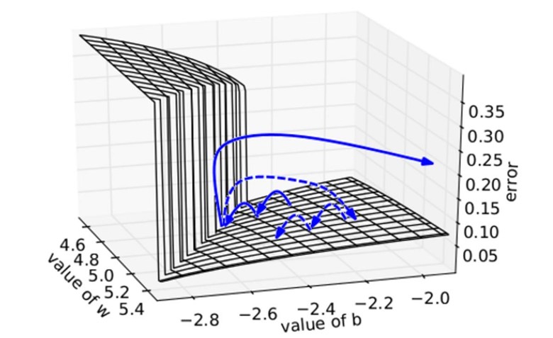
We plot the error surface of a one hidden unit recurrent network, highlighting the existence of high curvature walls. The solid lines depicts standard trajectories that gradient descent might follow. Using dashed arrow the diagram shows what would happen if the gradients is rescaled to a fixed size when its norm is above a threshold.
Source for the plot: Understanding the exploding gradient problem (Pascanu et al., 2012)