有些地方还没看懂, mark一下
文章来源: https://blog.csdn.net/g11d111/article/details/82855946
去年曾经使用过FCN(全卷积神经网络)及其派生Unet,再加上在爱奇艺的时候做过一些超分辨率重建的内容,其中用到了毕业于帝国理工的华人博士Shi Wenzhe(在Twitter任职)发表的PixelShuffle《Real-Time Single Image and Video Super-Resolution Using an Efficient Sub-Pixel Convolutional Neural Network
》的论文。PyTorch 0.4.1将这些上采样的方式定义为Vision Layers,现在对这4种在PyTorch中的上采样方法进行介绍。
0. 什么是上采样?
上采样,在深度学习框架中,可以简单的理解为**任何可以让你的图像变成更高分辨率的技术。**最简单的方式是重采样和插值:将输入图片input image进行rescale到一个想要的尺寸,而且计算每个点的像素点,使用如双线性插值bilinear等插值方法对其余点进行插值。
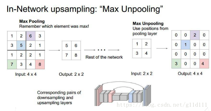
Unpooling是在CNN中常用的来表示max pooling的逆操作。这是从2013年纽约大学Matthew D. Zeiler和Rob Fergus发表的《Visualizing and Understanding Convolutional Networks》中引用的:因为max pooling不可逆,因此使用近似的方式来反转得到max pooling操作之前的原始情况:
记住max pooling做的时候的size,比如下图的一个4x4的矩阵,max pooling的size为2x2,stride为2,反卷积操作需要记住最大值的位置,将其余位置至为0就行。
Deconvolution(反卷积)在CNN中常用于表示一种反向卷积 ,但它并不是一个完全符合数学规定的反卷积操作。
与Unpooling不同,使用反卷积来对图像进行上采样是可以习得的。通常用来对卷积层的结果进行上采样,使其回到原始图片的分辨率。
反卷积也被称为分数步长卷积(convolution with fractional strides)或者转置卷积(transpose convolution)或者后向卷积backwards strided convolution。
真正的反卷积如wikipedia里面所说,但是不会有人在实际的CNN结构中使用它。
1. Vision Layer
在PyTorch中,上采样的层被封装在torch.nn中的Vision Layers里面,一共有4种:
- ① PixelShuffle
- ② Upsample
- ③ UpsamplingNearest2d
- ④ UpsamplingBilinear2d
下面,将对其分别进行说明
1.1 PixelShuffle
正常情况下,卷积操作会使feature map的高和宽变小。
但当我们的stride= 时,可以让卷积后的feature map的高和宽变大——即分辨率增大,这个新的操作叫做sub-pixel convolution,具体原理可以看PixelShuffle《Real-Time Single Image and Video Super-Resolution Using an Efficient Sub-Pixel Convolutional Neural Network
》的论文。
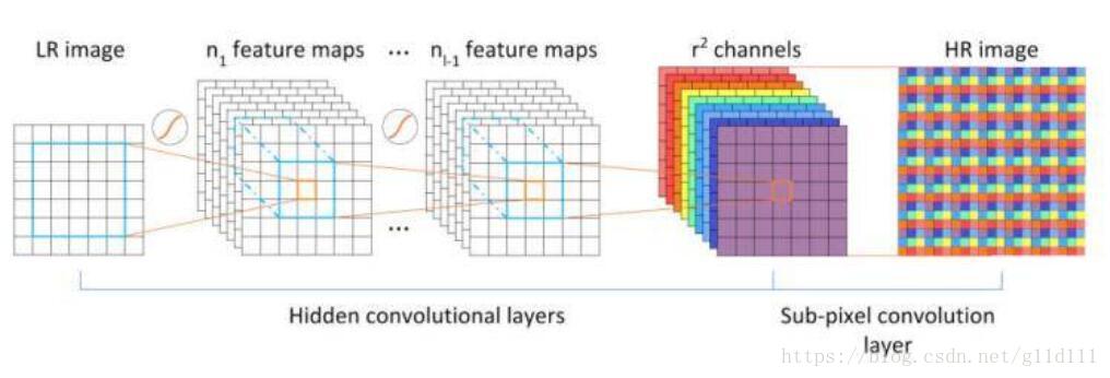
pixelshuffle算法的实现流程如上图,其实现的功能是:将一个H × W的低分辨率输入图像(Low Resolution),通过Sub-pixel操作将其变为rH x rW的高分辨率图像(High Resolution)。
但是其实现过程不是直接通过插值等方式产生这个高分辨率图像,而是通过卷积先得到个通道的特征图(特征图大小和输入低分辨率图像一致),然后通过周期筛选(periodic shuffing)的方法得到这个高分辨率的图像,其中为上采样因子(upscaling factor),也就是图像的扩大倍率。
定义
该类定义如下:
class torch.nn.PixleShuffle(upscale_factor)
- 1
- 1
这里的upscale_factor就是放大的倍数,数据类型为int。
以四维输入(N,C,H,W)为例,Pixelshuffle会将为(∗,,H,W)的Tensor给reshape成(∗,C,rH,rW)的Tensor。形式化地说,它的输入输出的shape如下:
- 输入: (N,C x upscale_factor,H,W)
- 输出: (N,C,H x upscale_factor,W x upscale_factor)
例子
>>> ps = nn.PixelShuffle(3)
>>> input = torch.tensor(1, 9, 4, 4)
>>> output = ps(input)
>>> print(output.size())
torch.Size([1, 1, 12, 12])
- 1
- 2
- 3
- 4
- 5
- 1
- 2
- 3
- 4
- 5
怎么样,是不是看起来挺简单的?我将在最后完整的介绍一下1)转置卷积 2)sub-pixel 卷积
3)反卷积以及pixelshuffle这几个知识点。
1.2 Upsample(新版本中推荐使用torch.nn.functional.interpolate)
对给定多通道的1维(temporal)、2维(spatial)、3维(volumetric)数据进行上采样。
对volumetric输入(3维——点云数据),输入数据Tensor格式为5维:minibatch x channels x depth x height x width
对spatial输入(2维——jpg、png等数据),输入数据Tensor格式为4维:minibatch x channels x height x width
对temporal输入(1维——向量数据),输入数据Tensor格式为3维:minibatch x channels x width
此算法支持最近邻,线性插值,双线性插值,三次线性插值对3维、4维、5维的输入Tensor分别进行上采样(Upsample)。
定义
该类定义如下:
class torch.nn.Upsample(size=None, scale_factor=None, mode='nearest', align_corners=None)
- 1
- 1
其中:
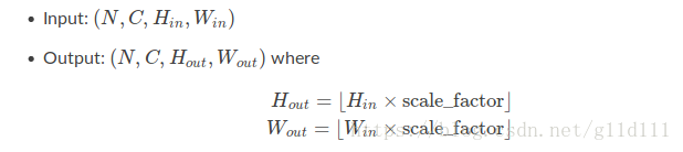
- size 是要输出的尺寸,数据类型为tuple: ([optional D_out], [optional H_out], W_out)
- scale_factor 在高度、宽度和深度上面的放大倍数。数据类型既可以是int——表明高度、宽度、深度都扩大同一倍数;亦或是tuple——指定高度、宽度、深度的扩大倍数。
- mode 上采样的方法,包括最近邻(nearest),线性插值(linear),双线性插值(bilinear),三次线性插值(trilinear),默认是最近邻(nearest)。
- align_corners 如果设为True,输入图像和输出图像角点的像素将会被对齐(aligned),这只在mode = linear, bilinear, or trilinear才有效,默认为False。
例子
>>> input = torch.arange(1, 5).view(1, 1, 2, 2).float()
>>> input
tensor([[[[ 1., 2.],
[ 3., 4.]]]])
>>> m = nn.Upsample(scale_factor=2, mode='nearest')
>>> m(input)
tensor([[[[ 1., 1., 2., 2.],
[ 1., 1., 2., 2.],
[ 3., 3., 4., 4.],
[ 3., 3., 4., 4.]]]])
>>> m = nn.Upsample(scale_factor=2, mode='bilinear') # align_corners=False
>>> m(input)
tensor([[[[ 1.0000, 1.2500, 1.7500, 2.0000],
[ 1.5000, 1.7500, 2.2500, 2.5000],
[ 2.5000, 2.7500, 3.2500, 3.5000],
[ 3.0000, 3.2500, 3.7500, 4.0000]]]])
>>> m = nn.Upsample(scale_factor=2, mode='bilinear', align_corners=True)
>>> m(input)
tensor([[[[ 1.0000, 1.3333, 1.6667, 2.0000],
[ 1.6667, 2.0000, 2.3333, 2.6667],
[ 2.3333, 2.6667, 3.0000, 3.3333],
[ 3.0000, 3.3333, 3.6667, 4.0000]]]])
>>> # Try scaling the same data in a larger tensor
>>>
>>> input_3x3 = torch.zeros(3, 3).view(1, 1, 3, 3)
>>> input_3x3[:, :, :2, :2].copy_(input)
tensor([[[[ 1., 2.],
[ 3., 4.]]]])
>>> input_3x3
tensor([[[[ 1., 2., 0.],
[ 3., 4., 0.],
[ 0., 0., 0.]]]])
>>> m = nn.Upsample(scale_factor=2, mode='bilinear') # align_corners=False
>>> # Notice that values in top left corner are the same with the small input (except at boundary)
>>> m(input_3x3)
tensor([[[[ 1.0000, 1.2500, 1.7500, 1.5000, 0.5000, 0.0000],
[ 1.5000, 1.7500, 2.2500, 1.8750, 0.6250, 0.0000],
[ 2.5000, 2.7500, 3.2500, 2.6250, 0.8750, 0.0000],
[ 2.2500, 2.4375, 2.8125, 2.2500, 0.7500, 0.0000],
[ 0.7500, 0.8125, 0.9375, 0.7500, 0.2500, 0.0000],
[ 0.0000, 0.0000, 0.0000, 0.0000, 0.0000, 0.0000]]]])
>>> m = nn.Upsample(scale_factor=2, mode='bilinear', align_corners=True)
>>> # Notice that values in top left corner are now changed
>>> m(input_3x3)
tensor([[[[ 1.0000, 1.4000, 1.8000, 1.6000, 0.8000, 0.0000],
[ 1.8000, 2.2000, 2.6000, 2.2400, 1.1200, 0.0000],
[ 2.6000, 3.0000, 3.4000, 2.8800, 1.4400, 0.0000],
[ 2.4000, 2.7200, 3.0400, 2.5600, 1.2800, 0.0000],
[ 1.2000, 1.3600, 1.5200, 1.2800, 0.6400, 0.0000],
[ 0.0000, 0.0000, 0.0000, 0.0000, 0.0000, 0.0000]]]])
- 1
- 2
- 3
- 4
- 5
- 6
- 7
- 8
- 9
- 10
- 11
- 12
- 13
- 14
- 15
- 16
- 17
- 18
- 19
- 20
- 21
- 22
- 23
- 24
- 25
- 26
- 27
- 28
- 29
- 30
- 31
- 32
- 33
- 34
- 35
- 36
- 37
- 38
- 39
- 40
- 41
- 42
- 43
- 44
- 45
- 46
- 47
- 48
- 49
- 50
- 51
- 52
- 53
- 54
- 55
- 56
- 1
- 2
- 3
- 4
- 5
- 6
- 7
- 8
- 9
- 10
- 11
- 12
- 13
- 14
- 15
- 16
- 17
- 18
- 19
- 20
- 21
- 22
- 23
- 24
- 25
- 26
- 27
- 28
- 29
- 30
- 31
- 32
- 33
- 34
- 35
- 36
- 37
- 38
- 39
- 40
- 41
- 42
- 43
- 44
- 45
- 46
- 47
- 48
- 49
- 50
- 51
- 52
- 53
- 54
- 55
- 56
1.3 UpsamplingNearest2d
本质上其实就是对jpg、png等格式图像数据的Upsample(mode='nearest')。
定义
class torch.nn.UpsamplingNearest2d(size=None, scale_factor=None)
- 1
- 1
输入输出:
例子
>>> input = torch.arange(1, 5).view(1, 1, 2, 2)
>>> input
tensor([[[[ 1., 2.],
[ 3., 4.]]]])
>>> m = nn.UpsamplingNearest2d(scale_factor=2)
>>> m(input)
tensor([[[[ 1., 1., 2., 2.],
[ 1., 1., 2., 2.],
[ 3., 3., 4., 4.],
[ 3., 3., 4., 4.]]]])
- 1
- 2
- 3
- 4
- 5
- 6
- 7
- 8
- 9
- 10
- 11
- 1
- 2
- 3
- 4
- 5
- 6
- 7
- 8
- 9
- 10
- 11
1.4 UpsamplingBilinear2d
跟1.3类似,本质上其实就是对jpg、png等格式图像数据的Upsample(mode='bilinear')。
定义
class torch.nn.UpsamplingBilinear2d(size=None, scale_factor=None)
- 1
- 1
输入输出:
例子
>>> input = torch.arange(1, 5).view(1, 1, 2, 2)
>>> input
tensor([[[[ 1., 2.],
[ 3., 4.]]]])
>>> m = nn.UpsamplingBilinear2d(scale_factor=2)
>>> m(input)
tensor([[[[ 1.0000, 1.3333, 1.6667, 2.0000],
[ 1.6667, 2.0000, 2.3333, 2.6667],
[ 2.3333, 2.6667, 3.0000, 3.3333],
[ 3.0000, 3.3333, 3.6667, 4.0000]]]])
- 1
- 2
- 3
- 4
- 5
- 6
- 7
- 8
- 9
- 10
- 11
- 1
- 2
- 3
- 4
- 5
- 6
- 7
- 8
- 9
- 10
- 11
2. 知识回顾
本段主要转自《一边Upsample一边Convolve:Efficient Sub-pixel-convolutional-layers详解
》
2.1 Transposed convolution(转置卷积)
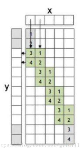
下面以一维向量进行卷积为例进行说明(stride=2),x为输入y为输出,通过1维卷积核/滤波器f来实现这个过程,x的size为8,f为[1, 2, 3, 4],y为5,x中灰色的方块表示用0进行padding。在f权重中的灰色方块代表f中某些值与x中的0进行了相乘。下图就是1维卷积的过程,从x到y。
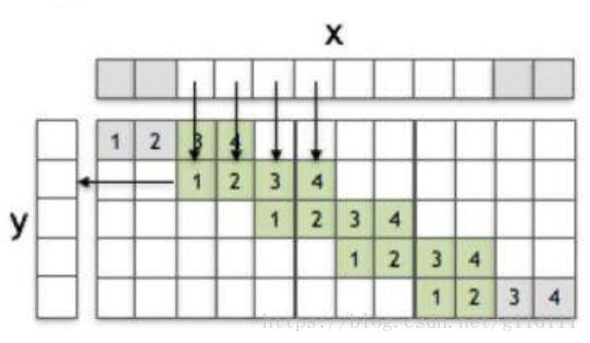
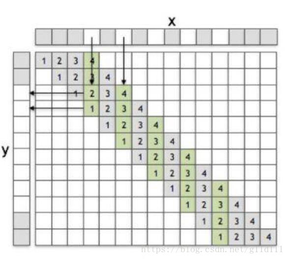
容易地,可以发现1维卷积的方式很直观,那么什么是转置卷积呢?故名思意,就是将卷积倒过来:
如上图所示,1维卷积核/滤波器被转过来了,这里进行一下额外的说明:
假设x = [, , …, ],y = [, , …, ],则最上面的白色块体对应的是。那么:
=
2.2 Sub-pixel convolution
还是以一维卷积为例,输入为x = [, , …, ],输出为y = [, , …, ]。sub-pixel convolution(stride=1/2)如图:
在1.1 PixelShuffle中说过,sub-pixel convolution的步长是介于0到1之间的,但是这个操作是如何实现的呢?简而言之,分为两步:
- ① 将stride设为1
- ② 将输入数据dilation(以stride=1/2为例,sub-pixel是将输入x的元素之间插入一些元素0,并在前后补上一些元素0),或者说根据分数索引(fractional indices)重新创建数据的排列形式。
2.3 Deconvolution
这里以2维卷积来进行演示,输入一个4 x 4的单通道图像,卷积核取1个4 x 4的,假设这里取上采样比例为2,那么我们的目标就是恢复成一个8 x 8的单通道图像。
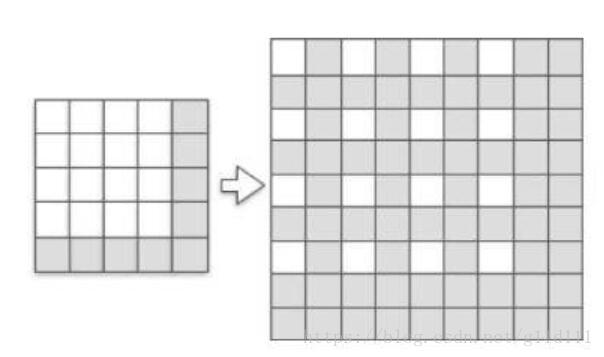
如上图,我们首先通过fractional indices从原input中创建一个sub-pixel图像,其中白色的像素点就是原input中的像素(在LR sapce中),灰色像素点则是通过zero padding而来的。
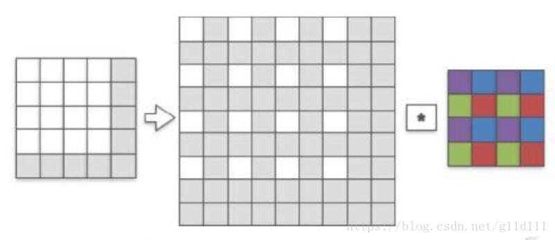
用一个4 x 4的卷积核来和刚才生成的sub-pixel图像进行stride=1的卷积,首先发现卷积核和sub-pixel图像中非零的像素进行了第一次有效卷积(图中紫色像素代表被激活的权重),然后我们将sub-pixels整体向右移动一格,让卷积核再进行一次卷积操作,会发现卷积核中蓝色像素的权重被激活,同理绿色和红色(注意这里是中间的那个8×8的sub-pixel图像中的白色像素点进行移动,而每次卷积的方式都相同)。
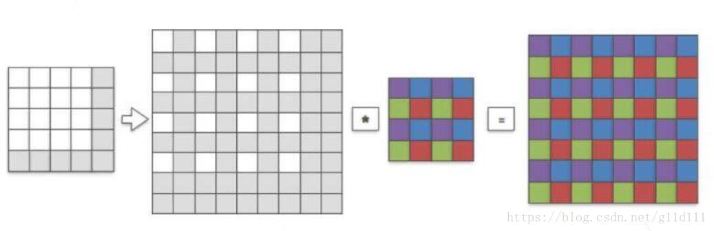
最后我们输出得到8 x 8的高分辨率图像(HR图像),HR图像和sub-pixel图像的大小是一致的,我们将其涂上颜色,颜色代表卷积核中权重和sub-pixel图像中哪个像素点进行了卷积(也就是哪个权重对对应的像素进行了贡献)。
Deconvlution的动态过程可见我之前翻译过的一篇文章《CNN概念之上采样,反卷积,Unpooling概念解释》
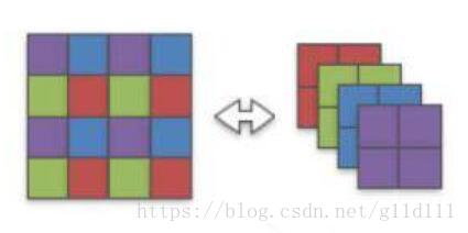
显然,我们可以看出,紫、蓝、绿、红四部分是相互独立的,那么,可以将这个4 x 4的卷积核分成4个2 x 2的卷积核如下:
注意,这个操作是可逆的。因为每个卷积权重在操作过程中都是独立的。
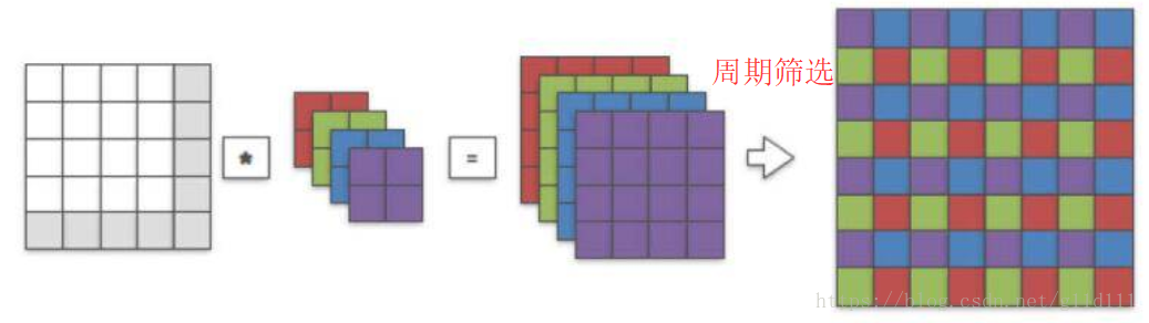
因此,我们可以直接对原始图像(未经过sub-pixel处理)直接进行2 x 2的卷积,并对输出进行周期筛选(periodic shuffling)来得到同样的8 x 8的高分辨率图像。
3. 说明
在新版本PyTorch中,这些插值Vision Layer都不推荐使用了,官方的说法是将其放在了torch.nn.functional.interpolate中,用此方法可以更个性化的定制用户的上采样或者下采样的需求。
4. 参考资料
[1] 一边Upsample一边Convolve:Efficient Sub-pixel-convolutional-layers详解
[2] 双线性插值(Bilinear Interpolation)
[3] torch.nn.functional.interpolate说明
[4] PyTorch 0.4.1——Vision layers
</div>