原文出处https://blog.csdn.net/qq_37366291/article/details/79832886
例子1
作用:使用傅里叶变换找出隐藏在噪声中的信号的频率成分。(指定信号的参数,采样频率为1 kHz,信号持续时间为1秒。)
Fs = 1000; % 采样频率
T = 1/Fs; % 采样周期
L = 1000; % 信号长度
t = (0:L-1)*T; % 时间向量
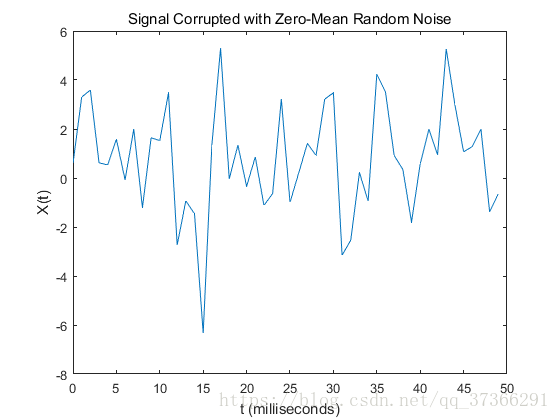
%%形成一个信号,包含振幅为0.7的50hz正弦信号和振幅为1的120hz正弦信号。
S = 0.7*sin(2*pi*50*t) + sin(2*pi*120*t);
X = S + 2*randn(size(t)); %用零均值的白噪声破坏信号,方差为4。
plot(1000*t(1:50),X(1:50))
title('Signal Corrupted with Zero-Mean Random Noise')
xlabel('t (milliseconds)')
ylabel('X(t)')1234567891011121314
由上图可知:从时域中我们很难观察到信号的频率成分。怎么办呢?当然使用强大的傅里叶变换。
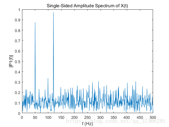
Y = fft(X);     %计算傅里叶变换,X是加噪后的信号

%%
%计算双边谱P2。然后计算基于P2的单面谱P1和偶值信号长度L。(不太理解。。。)
P2 = abs(Y/L);
P1 = P2(1:L/2+1);
P1(2:end-1) = 2*P1(2:end-1);

%%
%定义频率域f并绘制单面振幅谱P1。由于增加的噪音,振幅不完全是0.7和1。平均而言,较长的信号产生更好的频率近似。
f = Fs*(0:(L/2))/L;
plot(f,P1)
title('Single-Sided Amplitude Spectrum of X(t)')
xlabel('f (Hz)')
ylabel('|P1(f)|')123456789101112131415
%%
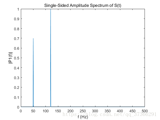
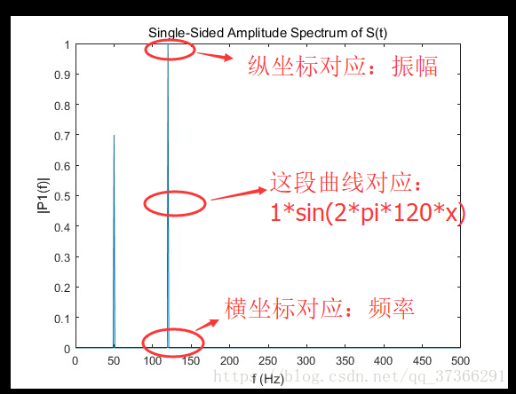
%现在,对原始的,未被损坏的信号进行傅里叶变换,并得到准确的振幅,0.7和1.0。
Y = fft(S); %S时原始的,没有加噪的信号。
P2 = abs(Y/L);
P1 = P2(1:L/2+1);
P1(2:end-1) = 2*P1(2:end-1);
plot(f,P1)
title('Single-Sided Amplitude Spectrum of S(t)')
xlabel('f (Hz)')
ylabel('|P1(f)|')1234567891011
加上一点自己的理解。
例子2
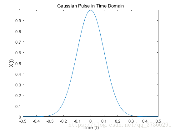
作用:利用傅里叶变换,将高斯脉冲从时域转换为频域。
Fs = 100;           % Sampling frequency
t = -0.5:1/Fs:0.5;  % Time vector
L = length(t);      % Signal length

X = 1/(4*sqrt(2*pi*0.01))*(exp(-t.^2/(2*0.01)));

plot(t,X)
title('Gaussian Pulse in Time Domain')
xlabel('Time (t)')
ylabel('X(t)')12345678910
%%
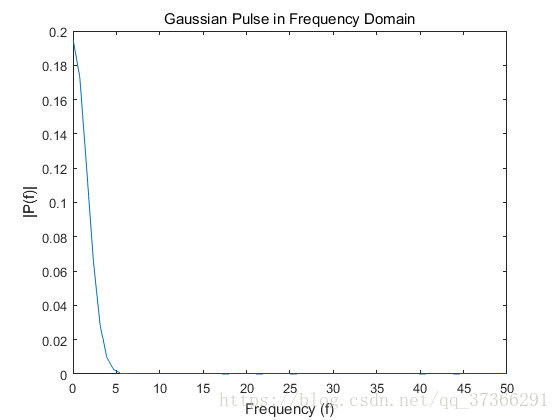
%要使用fft函数将信号转换为频域,首先要确定一个新的输入长度,该输入长度是原信号长度的下一个2次方。
%为了提高fft的性能,这将使信号X以尾随零的形式出现。
n = 2^nextpow2(L);
Y = fft(X,n);
f = Fs*(0:(n/2))/n;
P = abs(Y/n);
plot(f,P(1:n/2+1))
title('Gaussian Pulse in Frequency Domain')
xlabel('Frequency (f)')
ylabel('|P(f)|')12345678910111213
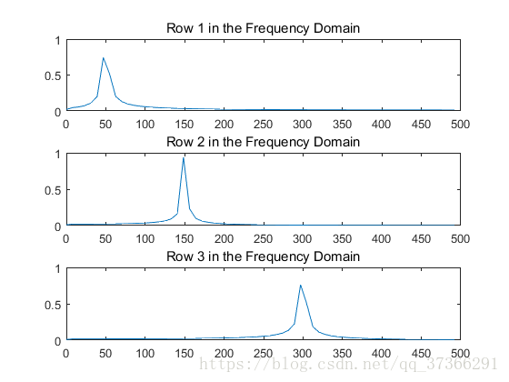
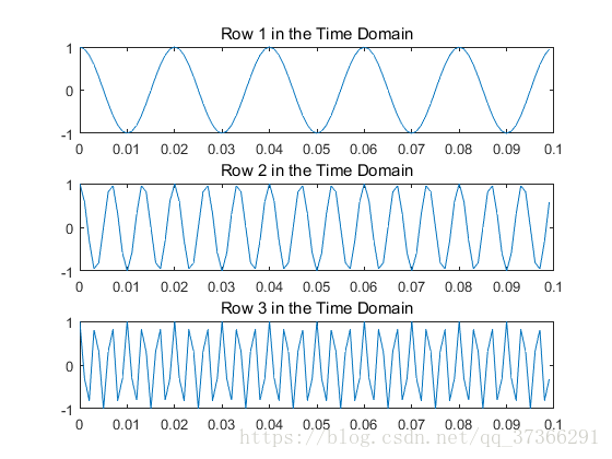
例子3余弦波
比较时域和频域的余弦波。指定信号的参数,采样频率为1kHz,信号持续时间为1秒。
Fs = 1000;                    % Sampling frequency
T = 1/Fs;                     % Sampling period
L = 1000;                     % Length of signal
t = (0:L-1)*T;                % Time vector

x1 = cos(2*pi*50*t);          % First row wave
x2 = cos(2*pi*150*t);         % Second row wave
x3 = cos(2*pi*300*t);         % Third row wave

X = [x1; x2; x3];

for i = 1:3
    subplot(3,1,i)
    plot(t(1:100),X(i,1:100))
    title(['Row ',num2str(i),' in the Time Domain'])
end12345678910111213141516
n = 2^nextpow2(L);
dim = 2;
Y = fft(X,n,dim);
P2 = abs(Y/n);
P1 = P2(:,1:n/2+1);
P1(:,2:end-1) = 2*P1(:,2:end-1);
for i=1:3
    subplot(3,1,i)
    plot(0:(Fs/n):(Fs/2-Fs/n),P1(i,1:n/2))
    title(['Row ',num2str(i), ' in the Frequency Domain'])
end1234567891011