学习stanford的课程http://ufldl.stanford.edu/wiki/index.php/UFLDL_Tutorial 一个月以来,对算法一知半解,Exercise也基本上是复制别人代码,现在想总结一下相关内容
1. Autoencoders and Sparsity
稀释编码:Sparsity parameter
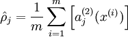
隐藏层的平均激活参数为
约束为

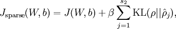
为实现这个目标,在cost Function上额外加上一项惩罚系数
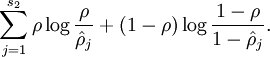
当此项达到最小值
此时cost Function
同时为了方便编程,将隐藏层时的后向传播参数也增加一项
为了得到Sparsity parameter,先对所有训练数据进行前向步骤,从而得到激活参数,再次前向步骤,进行反向传播调参,也就是要对所有训练数据进行两次的前向步骤
2.Backpropagation Algorithm
在计算过程中,简化了计算步骤
对于训练集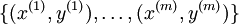 ,cost Function如下
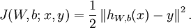
仅含方差项
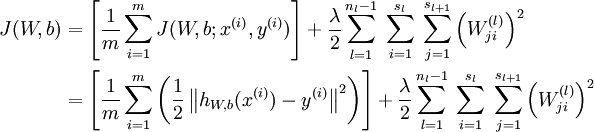
第一部分是方差,第二部分是规范化项,也称为weight decay项,此公式为overall cost function
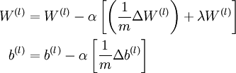
参数W,b的迭代公式如下
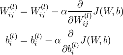
α为学习率
那么,backpropagation algorithm在参数计算中极大提高了效率
目的:梯度下降法,迭代多次,得到优化参数
每次迭代都计算cost function和gradient,再进行下一次迭代
BP 前向传播后,定义误差项1.输出层是对cost function 对输出结果求导2.中间层 下一层误差项与网络系数相乘,实现逆向推导
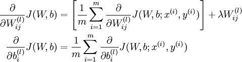
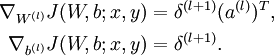
cost function分别对W,b求导如下
首先,对训练对象进行前向网络激活运算,得到网络输入值hW,b(x)
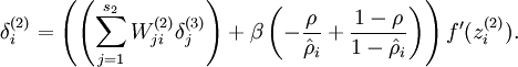
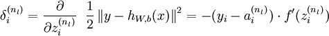
接着,对网络层l 中每一个节点i ,计算误差项 ,衡量该节点对于输出的误差所占权重,可用网络激活输出值与真实目标值之差来定义
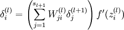
 ,nl 是输出层,对于隐藏层,则用
 作为输出的误差项的权重比来定义
算法步骤如下
- Perform a feedforward pass, computing the activations for layers L2, L3, and so on up to the output layer
 .
. - For each output unit i in layer nl (the output layer), set
- For

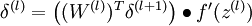
- For each node i in layer l, set
- For each node i in layer l, set
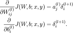
- Compute the desired partial derivatives, which are given as:
对于矩阵,在MATLAB中如下
- Perform a feedforward pass, computing the activations for layers
 ,
,  , up to the output layer
  , using the equations defining the forward propagation steps
 - For the output layer (layer
 ), set
 - For

- Set
- Set
- Compute the desired partial derivatives:

注: 为sigmoid函数,则
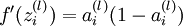
在此基础上,梯度下降算法gradient descent algorithm步骤如下
- Set
 ,
,  (matrix/vector of zeros) for all
  .
. - For
 to
to  ,
,- Use backpropagation to compute
 and
and  .
. - Set
 .
. - Set
 .
.
- Use backpropagation to compute
- Update the parameters:
3.Visualizing a Trained Autoencoder
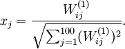
用pixel intensity values可视化编码器
已知输出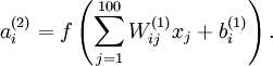
约束
定义pixel  (for all 100 pixels,
  )
)