一些问题:
1. 什么时候我的问题可以用GLM,什么时候我的问题不能用GLM?
2. GLM到底能给我们带来什么好处?
3. 如何评价GLM模型的好坏?
广义线性回归啊,虐了我快几个月了,还是没有彻底搞懂,看paper看代码的时候总是一脸懵逼。
大部分分布都能看作是指数族分布,广义差不多是这个意思,我们常见的线性回归和logistic回归都是广义线性回归的特例,可以由它推到出来。
参考:线性回归、logistic回归、广义线性模型——斯坦福CS229机器学习个人总结(一)
对着上面的教程,手写了一遍所有的公式,大致能理解其中的40%吧。
1. 线性回归和logistic回归都有概率形式,只是基础的分布假设不一样。线性回归假设误差y服从高斯分布;logistic回归假设y服从伯努利分布。有了分布形式,根据最大似然方法我们就很容易得到优化目标,这正好也推到出了我们用在线性回归中的最小二乘公式。
2. 在优化时所用的方法,梯度下降、梯度上升、牛顿法。梯度法的核心就是导数,我们优化的函数就是关于参数的函数,求导得斜率,走一步alpha,更新参数,迭代进行,即可得局部最优参数。
3. GLM的核心就是y服从的分布可以表示为指数分布族的形式,就可以推广线性模型的应用范围。logistic回归就是线性回归的推广。
那么如何根据指数分布族来构建广义线性模型呢?
啊哈,百度里讲GLM理论的不少(讲得也是比较粗糙),实例的几乎没有。下面是一个GLM在医学fMRI上的应用。
Statistical Analysis: The General Linear Model
What does a generalized linear model do? R
The overall summary is: You can first try linear regression. If this is not appropriate for your problem you can then try pre-transforming your y-data (a log-like or logit transform) and seeing if that fits better. However, if you transform your y-data you are using a new error model (in the transformed space such as log(y)-units instead of y-units, this can be better or can be worse depending on your situation). If this error model is not appropriate you can move on to a generalized linear model. However, the generalized linear model does not minimize square error in y-units but maximizes data likelihood under the chosen model. The distinction is mostly technical and maximum likelihood is often a good objective (so you should be willing to give up your original square-loss objective). If you wan’t to go further still you can try a generalized additive model which in addition to re-shaping the y distribution uses splines to learn re-shapings of the x-data.
“并不是说把推导什么的都放上来,那样不如干脆推荐读者看书好了。把指数分布族的形式写出来的话,这件事情会明了许多,比如为什么Logistic回归经常用logit联接函数(我见过一些民科的吐血解释)、为什么那个散布参数是个“讨厌参数”(极大似然估计可以扔掉它不管),等等。更深层的意义在于,广义线性模型不是简单的推广分布族,它是另一种思想。普通的回归的中心是加性误差,而GLM则是把模型分成两个组成成分来考虑,一个系统成分(自变量线性组合),一个随机成分(因变量的概率分布),二者用连接函数连起来。你可以说GLM是普通回归的推广,但我觉得这样有点低估它在统计建模思想上的突破。”
学习GLM的时候在网上找不到比较通俗易懂的教程。这里以一个实例应用来介绍GLM。
We used a Bayesian generalized linear model (GLM) to assign every gene to one or more cell populations, as previously described (Zeisel et al., 2015).
在单细胞RNA-seq的分析中,可以用GLM来寻找marker。
贝叶斯 + 广义 + 线性回归
线性回归:这个最基础,大部分人应该都知道。为什么找marker问题可以转化为线性回归问题?我们可以把每一个基因的表达当作自变量,把最终的类别作为因变量,拟合线性模型,然后根据系数的分布来得到marker。
广义:因变量(响应变量)可以服从多种分布(思考:为什么下文要用负二项分布);
贝叶斯:是一种新的思维方式,所有的系数都有自己的分布。
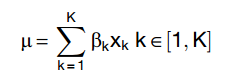
The GLM models the measured gene expression of a cell as realizations of a Negative Binomial probability distribution whose mean is determined by a linear combination of K predictors xi with coefficient bi.
For each cell, the outcome and predictors are known and the aim is to determine the posterior probability distributions of the coefficients.
As predictors, we use a continuous Baseline predictor and a categorical Cell Type predictor. The Baseline predictor value is the cell’s molecule count normalized to the average molecule count of all cells and takes account of the fact that we expect every gene to have a baseline expression proportional to the total number of expressed molecules within a particular cell. While the Cell Type predictor is set to 1 for the cluster BackSPIN assignation of the cell, and 0 for the other classes. From the definition of the model it follows that the coefficient bk for a Cell Type predictor xk can be interpreted as the additional number of molecules of a particular gene that are present as a result of the cell being of cell type k. A more detailed description of the model, including explanation of the prior probabilities used for the fitting as well as the full source code of the model, is provided elsewhere (Zeisel et al., 2015). The Stan (http://mc-stan.org) source is copied below for completeness:
data {
int < lower = 0 > N; # number of outcomes
int < lower = 0 > K; # number of predictors
matrix < lower = 0 > [N,K] x; # predictor matrix
int y[N]; # outcomes
}
parameters {
vector < lower = 1 > [K] beta; # coefficients
real < lower = 0.001 > r; # overdispersion
}
model {
vector < lower = 0.001 > [N] mu;
vector < lower = 1.001 > [N] rv;
# priors
r !cauchy(0, 1);
beta !pareto(1, 1.5);
# vectorize the overdispersion
for (n in 1:N) {
rv[n] < - square(r + 1) - 1;
}
# regression
mu < - x * (beta - 1) + 0.001;
y !neg_binomial(mu ./ rv, 1 / rv[1]);
}
To determine which genes are higher than basal expression in each population we compared the posterior probability distributions of the Baseline coefficient and the Cell Type coefficient. A gene was considered as marking a cell population if (1) its cell-typespecific coefficient exceeded the Baseline coefficient with 99.8% (95% for the mouse adult) posterior probability, and (2) the median of its posterior distribution did not fall below a threshold q set to 35% of the median posterior probability of the highest expressing group, and (3) the median of the highest-expressing cell type was greater than 0.4. For every gene this corresponds to a binary pattern (0 if the conditions are not met and 1 if they are), and genes can therefore be grouped according to their binarized expression patterns.
We use those binarized patterns to call transcription factor specificity. Our definition of a transcription factor gene was based of annotations provided by the merged annotation of PANTHER GO (Mi et al., 2013) and FANTOM5 (Okazaki et al., 2002), this list was further curated and missing genes and occasional misannotations corrected.
The feature selection procedure is based on the largest difference between the observed coefficient of variation (CV) and the predicted CV (estimated by a non-linear noise model learned from the data) See Figure S1C. In particular, Support Vector Regression (SVR, Smola and Vapnik, 1997) was used for this purpose (scikit-learn python implementation, default parameters with gamma = 0.06; Pedregosa et al., 2011).
特征选取:寻找观察CV值和预测CV值之间的最大差异。
SVR支持向量回归
Similarities between clusters within a species were summarized using a Pearson’s correlation coefficient calculated on the binarized matrix (Figures 1C and 1D).
The negative binomial-Lindley generalized linear model: Characteristics and application using crash data
这篇文章不错,可以仔细研读。
最新的Nature文章,有用GLM来做normalization的。
However, for Drop-seq, in which the number of UMIs is low per cell compared to the number of genes present, the set of genes detected per cell can be quite different. Hence, we normalize the expression of each gene separately by modelling the UMI counts as coming from a generalized linear model with negative binomial distribution, the mean of which can be dependent on technical factors related to sequencing depth. Specifically, for every gene we model the expected value of UMI counts as a function of the total number of reads assigned to that cell, and the number of UMIs per detected gene (sum of UMI divided by number of unique detected genes).
To solve the regression problem, we use a generalized linear model (glm function of base R package) with a regularized overdispersion parameter theta. Regularizing theta helps us to avoid overfitting which could occur for genes whose variability is mostly driven by biological processes rather than sampling noise and dropout events. To learn a regularized theta for every gene, we perform the following procedure.
1) For every gene, obtain an empirical theta using the maximum likelihood model (theta.ml function of the MASS R package) and the estimated mean vector that is obtained by a generalized linear model with Poisson error distribution.
2) Fit a line (loess, span = 0.33, degree = 2) through the variance–mean UMI count relationship (both log10transformed) and predict regularized theta using the fit. The relationship between variance and theta and mean is given by variance= mean + (mean2/theta).
Normalized expression is then defined as the Pearson residual of the regression model, which can be interpreted as the number of standard deviations by which an observed UMI count was higher or lower than its expected value. Unless stated otherwise, we clip expression to the range [-30, 30] to prevent outliers from dominating downstream analyses.