https://www.cnblogs.com/jins-note/p/11203934.html
Image Registration is a fundamental step in Computer Vision. In this article, we present OpenCV feature-based methods before diving into Deep Learning.
What is Image Registration?
Image registration is the process of transforming different images of one scene into the same coordinate system. These images can be taken at different times (multi-temporal registration), by different sensors (multi-modal registration), and/or from different viewpoints. The spatial relationships between these images can be rigid (translations and rotations), affine (shears for example), homographies, or complex large deformations models.

Image registration has a wide variety of applications: it is essential as soon as the task at hand requires comparing multiple images of the same scene. It is very common in the field of medical imagery, as well as for satellite image analysis and optical flow.
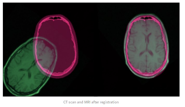
In this article, we will focus on a few different ways to perform image registration between a reference image and a sensed image. We choose not to go into iterative / intensity-based methods because they are less commonly used.
Traditional Feature-based Approaches
Since the early 2000s, image registration has mostly used traditional feature-based approaches. These approaches are based on three steps:Keypoint Detection and Feature Description, Feature Matching, and Image Warping. In brief, we select points of interest in both images, associate each point of interest in the reference image to its equivalent in the sensed image and transform the sensed image so that both images are aligned.
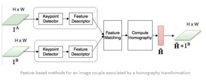
A keypoint is a point of interest. It defines what is important and distinctive in an image (corners, edges, etc). Each keypoint is represented by a descriptor: a feature vector containing the keypoints’ essential characteristics. A descriptor should be robust against image transformations (localization, scale, brightness, etc). Many algorithms perform keypoint detection and feature description:
- SIFT (Scale-invariant feature transform) is the original algorithm used for keypoint detection but it is not free for commercial use. The SIFT feature descriptor is invariant to uniform scaling, orientation, brightness changes, and partially invariant to affine distortion.
- SURF (Speeded Up Robust Features) is a detector and descriptor that is greatly inspired by SIFT. It presents the advantage of being several times faster. It is also patented.
- ORB (Oriented FAST and Rotated BRIEF) is a fast binary descriptor based on the combination of the FAST (Features from Accelerated Segment Test) keypoint detector and the BRIEF (Binary robust independent elementary features) descriptor. It is rotation invariant and robust to noise. It was developed in OpenCV Labs and it is an efficient and free alternative to SIFT.
- AKAZE (Accelerated-KAZE) is a sped-up version of KAZE. It presents a fast multiscale feature detection and description approach for non-linear scale spaces. It is both scale and rotation invariant. It is also free!
These algorithms are all available and easily usable in OpenCV. In the example below, we used the OpenCV implementation of AKAZE. The code remains roughly the same for the other algorithms: only the name of the algorithm needs to be modified.
import numpy as np
import cv2 as cv

img = cv.imread('image.jpg')
gray= cv.cvtColor(img, cv.COLOR_BGR2GRAY)

akaze = cv.AKAZE_create()
kp, descriptor = akaze.detectAndCompute(gray, None)

img=cv.drawKeypoints(gray, kp, img)
cv.imwrite('keypoints.jpg', img)

Feature Matching
Once keypoints are identified in both images that form a couple, we need to associate, or “match”, keypoints from both images that correspond in reality to the same point. One possible method is BFMatcher.knnMatch(). This matcher measures the distance between each pair of keypoint descriptors and returns for each keypoint its k best matches with the minimal distance.
We then apply a ratio filter to only keep the correct matches. In fact, to achieve a reliable matching, matched keypoints should be significantly closer than the nearest incorrect match.
import numpy as np
import cv2 as cv
import matplotlib.pyplot as plt

img1 = cv.imread('image1.jpg', cv.IMREAD_GRAYSCALE)  # referenceImage
img2 = cv.imread('image2.jpg', cv.IMREAD_GRAYSCALE)  # sensedImage

# Initiate AKAZE detector
akaze = cv.AKAZE_create()
# Find the keypoints and descriptors with SIFT
kp1, des1 = akaze.detectAndCompute(img1, None)
kp2, des2 = akaze.detectAndCompute(img2, None)

# BFMatcher with default params
bf = cv.BFMatcher()
matches = bf.knnMatch(des1, des2, k=2)

# Apply ratio test
good_matches = []
for m,n in matches:
    if m.distance < 0.75*n.distance:
        good_matches.append([m])

# Draw matches
img3 = cv.drawMatchesKnn(img1,kp1,img2,kp2,good_matches,None,flags=cv.DrawMatchesFlags_NOT_DRAW_SINGLE_POINTS)
cv.imwrite('matches.jpg', img3)
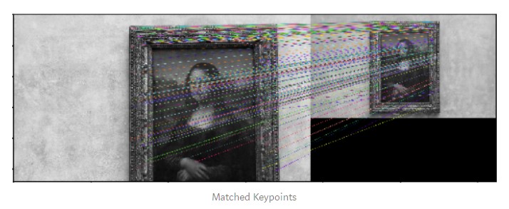
Check out this documentation for other feature matching methods implemented in OpenCV.
Image Warping
After matching at least four pairs of keypoints, we can transform one image relatively to the other one. This is called image warping. Any two images of the same planar surface in space are related by a homography. Homographies are geometric transformations that have 8 free parameters and are represented by a 3x3 matrix. They represent any distortion made to an image as a whole (as opposed to local deformations). Therefore, to obtain the transformed sensed image, we compute the homography matrix and apply it to the sensed image.
To ensure optimal warping, we use the RANSAC algorithm to detect outliers and remove them before determining the final homography. It is directly built-in OpenCV’s findHomography method. There exist alternatives to the RANSAC algorithm such as LMEDS: Least-Median robust method.
# Select good matched keypoints
ref_matched_kpts = np.float32([kp1[m[0].queryIdx].pt for m in good_matches]).reshape(-1,1,2)
sensed_matched_kpts = np.float32([kp2[m[0].trainIdx].pt for m in good_matches]).reshape(-1,1,2)

# Compute homography
H, status = cv.findHomography(ref_matched_kpts, sensed_matched_kpts, cv.RANSAC,5.0)

# Warp image
warped_image = cv.warpPerspective(img1, H, (img1.shape[1]+img2.shape[1], img1.shape[0]))

cv.imwrite('warped.jpg', warped_image)
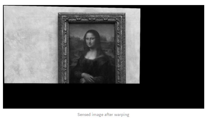
If you are interested in more details about these three steps, OpenCV has put together a series of useful tutorials.
Deep Learning Approaches
Most research nowadays in image registration concerns the use of deep learning. In the past few years, deep learning has allowed for state-of-the-art performance in Computer Vision tasks such as image classification, object detection, and segmentation. There is no reason why this couldn’t be the case for Image Registration.
Feature Extraction
The first way deep learning was used for image registration was for feature extraction. Convolutional neural networks’ successive layers manage to capture increasingly complex image characteristics and learn task-specific features. Since 2014, researchers have applied these networks to the feature extraction step rather than SIFT or similar algorithms.
- In 2014, Dosovitskiy et al. proposed a generic feature learning methodto train a convolutional neural network using only unlabeled data. The genericity of these features enabled them to be robust to transformations. These features, or descriptors, outperformed SIFT descriptors for matching tasks.
- In 2018, Yang et al. developed a non-rigid registration method based on the same idea. They used layers of a pre-trained VGG network to generate a feature descriptor that keeps both convolutional information and localization capabilities. These descriptors also seem to outperform SIFT-like detectors, particularly in cases where SIFT contains many outliers or cannot match a sufficient number of feature points.

The code for this last paper can be found here. While we were able to test this registration method on our own images within 15 minutes, the algorithm is approximatively 70 times slower than the SIFT-like methods implemented earlier in this article.
Homography Learning
Instead of limiting the use of deep learning to feature extraction, researchers tried to use a neural network to directly learn the geometric transformation to align two images.
Supervised Learning
In 2016, DeTone et al. published Deep Image Homography Estimation that describes Regression HomographyNet, a VGG style model that learns the homography relating two images. This algorithm presents the advantage of learning the homography and the CNN model parameters simultaneously in an end-to-end fashion: no need for the previous two-stage process!
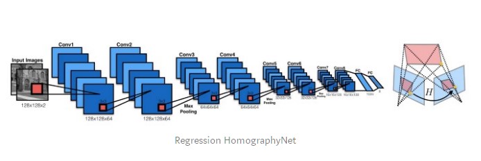
The network produces eight real-valued numbers as an output. It is trained in a supervised fashion thanks to a Euclidean loss between the output and the ground-truth homography.
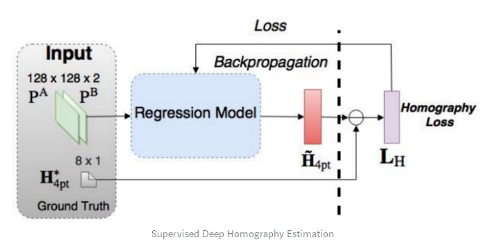
Like any supervised approach, this homography estimation method requires labeled pairs of data. While it is easy to obtain the ground truth homographies for artificial image pairs, it is much more expensive to do so on real data.
Unsupervised Learning
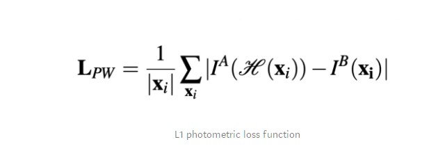
With this in mind, Nguyen et al. presented an unsupervised approach to deep image homography estimation. They kept the same CNN but had to use a new loss function adapted to the unsupervised approach: they chose the photometric loss that does not require a ground-truth label. Instead, it computes the similarity between the reference image and the sensed transformed image.
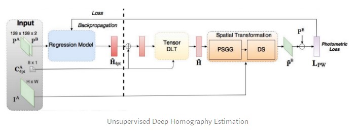
The authors claim that this unsupervised method obtains comparable or better accuracy and robustness to illumination variation than traditional feature-based methods, with faster inference speed. In addition, it has superior adaptability and performance compared to the supervised method.
Other Approaches
Reinforcement Learning
Deep
reinforcement learning is gaining traction as a registration method for
medical applications. As opposed to a pre-defined optimization
algorithm, in this approach, we use a trained agent to perform the registration.
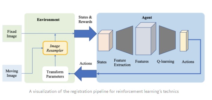
- In 2016, Liao et al. were the first to use reinforcement learning for image registration. Their method is based on a greedy supervised algorithm for end-to-end training. Its goal is to align the images by finding the best sequence of motion actions. This approach outperformed several state-of-the-art methods but it was only used for rigid transformations.
- Reinforcement Learning has also been used for more complex transformations. In Robust non-rigid registration through agent-based action learning, Krebs et al. apply an artificial agent to optimize the parameters of a deformation model. This method was evaluated on inter-subject registration of prostate MRI images and showed promising results in 2-D and 3-D.
Complex Transformations
A significant proportion of current research in image registration concerns the field of medical imagery. Often times, the transformation between two medical images cannot simply be described by a homography matrix because of the local deformations of the subject (due to breathing, anatomical changes, etc.). More
complex transformations models are necessary, such as diffeomorphisms
that can be represented by displacement vector fields.

Researchers have tried to use neural networks to estimate these large deformation models that have many parameters.
- A first example is Krebs et al.’s Reinforcement Learning method mentioned just above.
- In 2017 De Vos et al. proposed the DIRNet. It is a network that used a CNN to predict a grid of control points that are used to generate the displacement vector field to warp the sensed image according to the reference image.

- Quicksilver registration tackles a similar problem. Quicksilver uses a deep encoder-decoder network to predict patch-wise deformationsdirectly on image appearance.
We hope you enjoyed our article! Image registration is a vast field with numerous use cases. There is plenty of other fascinating research on this subject that we could not mention in this article, we tried to keep it to a few fundamental and accessible approaches. This survey on deep learning in Medical Image Registration could be a good place to look for more information.
