第八章 秩转换的非参数检验
非参数检验(nonparanmetric)是相对于参数检验(parametric test)而言的。
当总体分布不能有已知的数学形式表达、没有总体参数时,就谈不上参数检验。若两个或多个总体方差不等,也不能对其总体均数进行t
检验或F检验。
对于计量资料,不满足参数检验,可尝试1、变量变换,2、非参数检验。
对于等级资料,常用非参数检验。
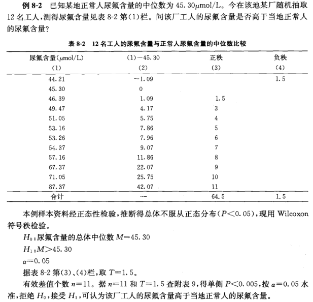
第一节 配对样本比较的wilcoxon 符号秩检验
用于配对样本差值的中位数与0的比较;
用于单个样本中位数和总体中位数比较。
8-2
> x<-c(44.21,45.30,46.39,49.47,51.05,53.16,53.26,54.37,57.16,67.37,71.05,87.37)
> wilcox.test(x,mu=45.3,al="greater")

	Wilcoxon signed rank test with continuity correction

data:  x
V = 65, p-value = 0.00255
alternative hypothesis: true location is greater than 45.3

Warning message:
In wilcox.test.default(x, mu = 45.3, al = "greater") :
  有0时无法計算精確的p值
> x<-c(44.21,45.30+1e-5,46.39,49.47,51.05,53.16,53.26,54.37,57.16,67.37,71.05,87.37)
> wilcox.test(x,mu=45.3,al="greater")

	Wilcoxon signed rank test

data:  x
V = 76, p-value = 0.0007324
alternative hypothesis: true location is greater than 45.3
两个独立样本比较的wilcoxon秩和检验
8-3

> library(DescTools)
> #检验方差齐性
> x<-c(2.78,3.23,4.2,4.87,5.12,6.21,7.18,8.05,8.56,9.6)
> y<-c(3.23,3.50,4.04,4.15,4.28,4.34,4.47,4.64,4.75,4.82,4.95,5.10)
> LeveneTest(c(x,y),factor(c(rep("x",length(x)),rep('y',length(y)))))
Levene's Test for Homogeneity of Variance (center = median)
      Df F value    Pr(>F)
group  1  18.865 0.0003152 ***
      20
---
Signif. codes:  0 ‘***’ 0.001 ‘**’ 0.01 ‘*’ 0.05 ‘.’ 0.1 ‘ ’ 1
> wilcox.test(x,y,al="greater")

	Wilcoxon rank sum test with continuity correction

data:  x and y
W = 86.5, p-value = 0.04318
alternative hypothesis: true location shift is greater than 0

Warning message:
In wilcox.test.default(x, y, al = "greater") : 无法精確計算带连结的p值
> wilcox.test(x,y,al="greater",exact = F)

	Wilcoxon rank sum test with continuity correction

data:  x and y
W = 86.5, p-value = 0.04318
alternative hypothesis: true location shift is greater than 0
8-4 非成对样本的秩次和检验 频数资料和等级资料的两样本比较

> x<-rep(1:5,c(1,8,16,10,4))
> y<-rep(1:5,c(2,23,11,4,0))
> x
 [1] 1 2 2 2 2 2 2 2 2 3 3 3 3 3 3 3 3 3 3 3 3 3 3 3 3 4 4 4 4 4 4 4 4 4 4 5 5 5 5
> y
 [1] 1 1 2 2 2 2 2 2 2 2 2 2 2 2 2 2 2 2 2 2 2 2 2 2 2 3 3 3 3 3 3 3 3 3 3 3 4 4 4 4
> sum(length(x))+sum(length(y))
[1] 79
> wilcox.test(x,y,al="greater")

	Wilcoxon rank sum test with continuity correction

data:  x and y
W = 1137, p-value = 0.000109
alternative hypothesis: true location shift is greater than 0

Warning message:
In wilcox.test.default(x, y, al = "greater") : 无法精確計算带连结的p值
> wilcox.test(x,y,al="greater",exact = F)

	Wilcoxon rank sum test with continuity correction

data:  x and y
W = 1137, p-value = 0.000109
alternative hypothesis: true location shift is greater than 0

> var.test(x,y) #两者方差比置信度为95%的置信区间为[0.9037,3.2584],因为1在置信区间中 认为两者方差相同

	F test to compare two variances

data:  x and y
F = 1.7137, num df = 38, denom df = 39, p-value = 0.0982
alternative hypothesis: true ratio of variances is not equal to 1
95 percent confidence interval:
 0.9037002 3.2584792
sample estimates:
ratio of variances
          1.713699
第三节 完全随机设计多个样本比较的Kruskal-waillis H 检验
> # 多个独立样本比较的kruskal-wallis H 检验
> #kruskal.test()是对两个以上样本进行比较的非参数检验方法
> # 又称为H检验,它对多个总体分布的形状差别不敏感,用于推断计量资料或等级资料的多个独立样本所来自的多个总体分布是否有差别
> #8-5

> # x 为列表时,g无效
> x<-c(32.5,35.5,40.5,46,49,16,20.5,22.5,29,36,6.5,9.0,12.5,18.0,24)
> x<-data.frame(x,g=rep(1:3,c(5,5,5)))
> x
      x g
1  32.5 1
2  35.5 1
3  40.5 1
4  46.0 1
5  49.0 1
6  16.0 2
7  20.5 2
8  22.5 2
9  29.0 2
10 36.0 2
11  6.5 3
12  9.0 3
13 12.5 3
14 18.0 3
15 24.0 3
> x<-as.list(x)
> x
$x
 [1] 32.5 35.5 40.5 46.0 49.0 16.0 20.5 22.5 29.0 36.0  6.5  9.0 12.5 18.0 24.0

$g
 [1] 1 1 1 1 1 2 2 2 2 2 3 3 3 3 3

> kruskal.test(x)

	Kruskal-Wallis rank sum test

data:  x
Kruskal-Wallis chi-squared = 22.069, df = 1, p-value = 2.631e-06

> #x为向量,g
> meidingluo<-data.frame(
+ x<-c(32.5,35.5,40.5,46,49,16,20.5,22.5,29,36,6.5,9.0,12.5,18.0,24),
+ g<-factor(rep(1:3,c(5,5,5)))
+ )
> kruskal.test(x~g,meidingluo)

	Kruskal-Wallis rank sum test

data:  x by g
Kruskal-Wallis chi-squared = 9.74, df = 2, p-value = 0.007673

> # 两种计算结果P值不同