Pipelines and composite estimators
https://scikit-learn.org/stable/modules/compose.html
转换器通常跟分类器、回归器、其它的估计器组合使用,构建一个组合的估计器。(可以理解为 组合模型)
这就叫流水线技术Pipeline。
流水线中常常和 特征联合(FeatureUnion) 工具组合使用, 特征联合工具连接 不同转换器的输出, 组成组合的特征空间。
另外,转化的特征回归器(TransformedTargetRegressor),仅仅处理转换目标,相对地, 流水线仅仅转换特征数据。
Transformers are usually combined with classifiers, regressors or other estimators to build a composite estimator. The most common tool is a Pipeline. Pipeline is often used in combination with FeatureUnion which concatenates the output of transformers into a composite feature space. TransformedTargetRegressor deals with transforming the target (i.e. log-transform y). In contrast, Pipelines only transform the observed data (X).
Pipeline: chaining estimators
流水线工具可以连接多个估计器成为一个估计器。
这是非常有用的,因为在机器学习中经常有固定的步骤顺序, 例如 处理数据-》特征提取 -》正则化 -》分类。
流水线的设计有多个目的:
(1)封装和便利。 对处理流程的封装, 达到使用上便利的目的。
组合后的估计器用户向正常模型一样,只需要关注 fit predict接口。 将原始数据和目标 输入模型,使用predict接口预测新的数据。
(2)联合参数选择。对流水线上的所有转换器和估计器进行参数选择。
(3)安全性。 特别是对交叉验证,不会漏数据。
Pipelinecan be used to chain multiple estimators into one. This is useful as there is often a fixed sequence of steps in processing the data, for example feature selection, normalization and classification.Pipelineserves multiple purposes here:
- Convenience and encapsulation
You only have to call fit and predict once on your data to fit a whole sequence of estimators.
- Joint parameter selection
You can grid search over parameters of all estimators in the pipeline at once.
- Safety
Pipelines help avoid leaking statistics from your test data into the trained model in cross-validation, by ensuring that the same samples are used to train the transformers and predictors.
All estimators in a pipeline, except the last one, must be transformers (i.e. must have a transform method). The last estimator may be any type (transformer, classifier, etc.).
流水线API
两种构造流水线方式 : Pipeline 和 make_pipeline
The
Pipelineis built using a list of(key, value)pairs, where thekeyis a string containing the name you want to give this step andvalueis an estimator object:>>> from sklearn.pipeline import Pipeline >>> from sklearn.svm import SVC >>> from sklearn.decomposition import PCA >>> estimators = [('reduce_dim', PCA()), ('clf', SVC())] >>> pipe = Pipeline(estimators) >>> pipe Pipeline(steps=[('reduce_dim', PCA()), ('clf', SVC())])The utility function
make_pipelineis a shorthand for constructing pipelines; it takes a variable number of estimators and returns a pipeline, filling in the names automatically:>>> from sklearn.pipeline import make_pipeline >>> from sklearn.naive_bayes import MultinomialNB >>> from sklearn.preprocessing import Binarizer >>> make_pipeline(Binarizer(), MultinomialNB()) Pipeline(steps=[('binarizer', Binarizer()), ('multinomialnb', MultinomialNB())])
Pipelining: chaining a PCA and a logistic regression -- 流水线示例
https://scikit-learn.org/stable/auto_examples/compose/plot_digits_pipe.html#sphx-glr-auto-examples-compose-plot-digits-pipe-py
使用PCA方法,做高维数据的降维工作, 然后输出的特征做维 逻辑回归模型的输入。
并使用网格搜索, 做降维的目的维数的选择,和逻辑回归的参数选择。
The PCA does an unsupervised dimensionality reduction, while the logistic regression does the prediction.
We use a GridSearchCV to set the dimensionality of the PCA
Out:
Best parameter (CV score=0.920):
{'logistic__C': 0.046415888336127774, 'pca__n_components': 45}
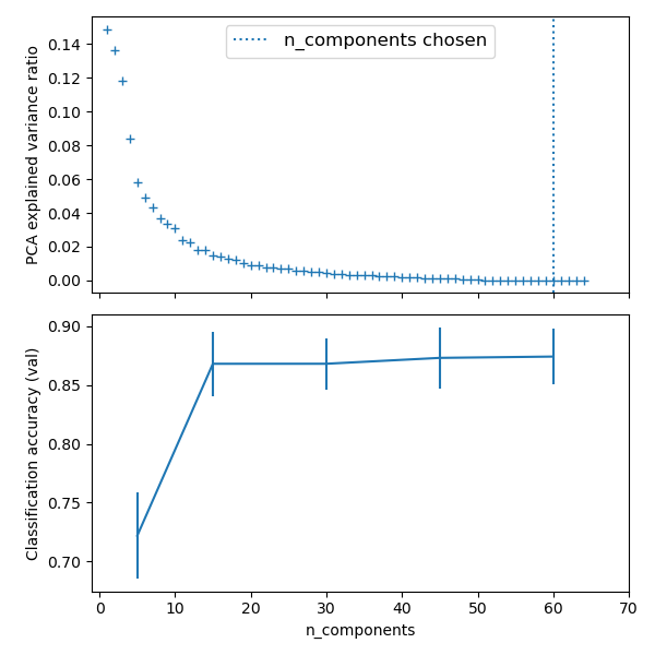
print(__doc__)


# Code source: Gaël Varoquaux
# Modified for documentation by Jaques Grobler
# License: BSD 3 clause


import numpy as np
import matplotlib.pyplot as plt
import pandas as pd

from sklearn import datasets
from sklearn.decomposition import PCA
from sklearn.linear_model import LogisticRegression
from sklearn.pipeline import Pipeline
from sklearn.model_selection import GridSearchCV


# Define a pipeline to search for the best combination of PCA truncation
# and classifier regularization.
pca = PCA()
# set the tolerance to a large value to make the example faster
logistic = LogisticRegression(max_iter=10000, tol=0.1)
pipe = Pipeline(steps=[('pca', pca), ('logistic', logistic)])

X_digits, y_digits = datasets.load_digits(return_X_y=True)

# Parameters of pipelines can be set using ‘__’ separated parameter names:
param_grid = {
    'pca__n_components': [5, 15, 30, 45, 64],
    'logistic__C': np.logspace(-4, 4, 4),
}
search = GridSearchCV(pipe, param_grid, n_jobs=-1)
search.fit(X_digits, y_digits)
print("Best parameter (CV score=%0.3f):" % search.best_score_)
print(search.best_params_)

# Plot the PCA spectrum
pca.fit(X_digits)

fig, (ax0, ax1) = plt.subplots(nrows=2, sharex=True, figsize=(6, 6))
ax0.plot(np.arange(1, pca.n_components_ + 1),
         pca.explained_variance_ratio_, '+', linewidth=2)
ax0.set_ylabel('PCA explained variance ratio')

ax0.axvline(search.best_estimator_.named_steps['pca'].n_components,
            linestyle=':', label='n_components chosen')
ax0.legend(prop=dict(size=12))

# For each number of components, find the best classifier results
results = pd.DataFrame(search.cv_results_)
components_col = 'param_pca__n_components'
best_clfs = results.groupby(components_col).apply(
    lambda g: g.nlargest(1, 'mean_test_score'))

best_clfs.plot(x=components_col, y='mean_test_score', yerr='std_test_score',
               legend=False, ax=ax1)
ax1.set_ylabel('Classification accuracy (val)')
ax1.set_xlabel('n_components')

plt.xlim(-1, 70)

plt.tight_layout()
plt.show()
SVM-Anova: SVM with univariate feature selection -- 流水线应用于特征选择
https://scikit-learn.org/stable/auto_examples/svm/plot_svm_anova.html#sphx-glr-auto-examples-svm-plot-svm-anova-py
对鸢尾花数据,4维度,增加36维度噪声特征。
然后使用 SelectPercentile 特征选择器,对特征筛选。
使用网格搜索, 按照特征覆盖度(特征分数从高到底的覆盖率),估算模型分数,确定最佳模型对应的特征覆盖度。
10维是峰值。
This example shows how to perform univariate feature selection before running a SVC (support vector classifier) to improve the classification scores. We use the iris dataset (4 features) and add 36 non-informative features. We can find that our model achieves best performance when we select around 10% of features.
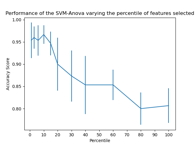
print(__doc__)

import numpy as np
import matplotlib.pyplot as plt
from sklearn.datasets import load_iris
from sklearn.feature_selection import SelectPercentile, chi2
from sklearn.model_selection import cross_val_score
from sklearn.pipeline import Pipeline
from sklearn.preprocessing import StandardScaler
from sklearn.svm import SVC


# #############################################################################
# Import some data to play with
X, y = load_iris(return_X_y=True)
# Add non-informative features
np.random.seed(0)
X = np.hstack((X, 2 * np.random.random((X.shape[0], 36))))

# #############################################################################
# Create a feature-selection transform, a scaler and an instance of SVM that we
# combine together to have an full-blown estimator
clf = Pipeline([('anova', SelectPercentile(chi2)),
                ('scaler', StandardScaler()),
                ('svc', SVC(gamma="auto"))])

# #############################################################################
# Plot the cross-validation score as a function of percentile of features
score_means = list()
score_stds = list()
percentiles = (1, 3, 6, 10, 15, 20, 30, 40, 60, 80, 100)

for percentile in percentiles:
    clf.set_params(anova__percentile=percentile)
    this_scores = cross_val_score(clf, X, y)
    score_means.append(this_scores.mean())
    score_stds.append(this_scores.std())

plt.errorbar(percentiles, score_means, np.array(score_stds))
plt.title(
    'Performance of the SVM-Anova varying the percentile of features selected')
plt.xticks(np.linspace(0, 100, 11, endpoint=True))
plt.xlabel('Percentile')
plt.ylabel('Accuracy Score')
plt.axis('tight')
plt.show()
SelectPercentile
https://scikit-learn.org/stable/modules/generated/sklearn.feature_selection.SelectPercentile.html
Select features according to a percentile of the highest scores.
选择前10得分的特征。
>>> from sklearn.datasets import load_digits
>>> from sklearn.feature_selection import SelectPercentile, chi2
>>> X, y = load_digits(return_X_y=True)
>>> X.shape
(1797, 64)
>>> X_new = SelectPercentile(chi2, percentile=10).fit_transform(X, y)
>>> X_new.shape
(1797, 7)
Sample pipeline for text feature extraction and evaluation -- 流水线示例,应用于文本特征抽取
https://scikit-learn.org/stable/auto_examples/model_selection/grid_search_text_feature_extraction.html#sphx-glr-auto-examples-model-selection-grid-search-text-feature-extraction-py
对20个新闻集团的数据集, 做特征提取(CountVectorizer TfidfTransformer),并嵌入到流水线中, 作为svm模型的输入。
The dataset used in this example is the 20 newsgroups dataset which will be automatically downloaded and then cached and reused for the document classification example.
You can adjust the number of categories by giving their names to the dataset loader or setting them to None to get the 20 of them.
Here is a sample output of a run on a quad-core machine:
Loading 20 newsgroups dataset for categories:
['alt.atheism', 'talk.religion.misc']
1427 documents
2 categories

Performing grid search...
pipeline: ['vect', 'tfidf', 'clf']
parameters:
{'clf__alpha': (1.0000000000000001e-05, 9.9999999999999995e-07),
 'clf__max_iter': (10, 50, 80),
 'clf__penalty': ('l2', 'elasticnet'),
 'tfidf__use_idf': (True, False),
 'vect__max_n': (1, 2),
 'vect__max_df': (0.5, 0.75, 1.0),
 'vect__max_features': (None, 5000, 10000, 50000)}
done in 1737.030s

Best score: 0.940
Best parameters set:
    clf__alpha: 9.9999999999999995e-07
    clf__max_iter: 50
    clf__penalty: 'elasticnet'
    tfidf__use_idf: True
    vect__max_n: 2
    vect__max_df: 0.75
    vect__max_features: 50000
# Author: Olivier Grisel <olivier.grisel@ensta.org>
#         Peter Prettenhofer <peter.prettenhofer@gmail.com>
#         Mathieu Blondel <mathieu@mblondel.org>
# License: BSD 3 clause
from pprint import pprint
from time import time
import logging

from sklearn.datasets import fetch_20newsgroups
from sklearn.feature_extraction.text import CountVectorizer
from sklearn.feature_extraction.text import TfidfTransformer
from sklearn.linear_model import SGDClassifier
from sklearn.model_selection import GridSearchCV
from sklearn.pipeline import Pipeline

print(__doc__)

# Display progress logs on stdout
logging.basicConfig(level=logging.INFO,
                    format='%(asctime)s %(levelname)s %(message)s')


# #############################################################################
# Load some categories from the training set
categories = [
    'alt.atheism',
    'talk.religion.misc',
]
# Uncomment the following to do the analysis on all the categories
#categories = None

print("Loading 20 newsgroups dataset for categories:")
print(categories)

data = fetch_20newsgroups(subset='train', categories=categories)
print("%d documents" % len(data.filenames))
print("%d categories" % len(data.target_names))
print()

# #############################################################################
# Define a pipeline combining a text feature extractor with a simple
# classifier
pipeline = Pipeline([
    ('vect', CountVectorizer()),
    ('tfidf', TfidfTransformer()),
    ('clf', SGDClassifier()),
])

# uncommenting more parameters will give better exploring power but will
# increase processing time in a combinatorial way
parameters = {
    'vect__max_df': (0.5, 0.75, 1.0),
    # 'vect__max_features': (None, 5000, 10000, 50000),
    'vect__ngram_range': ((1, 1), (1, 2)),  # unigrams or bigrams
    # 'tfidf__use_idf': (True, False),
    # 'tfidf__norm': ('l1', 'l2'),
    'clf__max_iter': (20,),
    'clf__alpha': (0.00001, 0.000001),
    'clf__penalty': ('l2', 'elasticnet'),
    # 'clf__max_iter': (10, 50, 80),
}

if __name__ == "__main__":
    # multiprocessing requires the fork to happen in a __main__ protected
    # block

    # find the best parameters for both the feature extraction and the
    # classifier
    grid_search = GridSearchCV(pipeline, parameters, n_jobs=-1, verbose=1)

    print("Performing grid search...")
    print("pipeline:", [name for name, _ in pipeline.steps])
    print("parameters:")
    pprint(parameters)
    t0 = time()
    grid_search.fit(data.data, data.target)
    print("done in %0.3fs" % (time() - t0))
    print()

    print("Best score: %0.3f" % grid_search.best_score_)
    print("Best parameters set:")
    best_parameters = grid_search.best_estimator_.get_params()
    for param_name in sorted(parameters.keys()):
        print("	%s: %r" % (param_name, best_parameters[param_name]))
Pipeline Anova SVM --- 选择最优若干特征
https://scikit-learn.org/stable/auto_examples/feature_selection/plot_feature_selection_pipeline.html#sphx-glr-auto-examples-feature-selection-plot-feature-selection-pipeline-py
使用anova做单变量特征选择,选择最优的3个,然后送入svm。
Simple usage of Pipeline that runs successively a univariate feature selection with anova and then a SVM of the selected features.
Using a sub-pipeline, the fitted coefficients can be mapped back into the original feature space.
Out:
              precision    recall  f1-score   support

           0       0.75      0.50      0.60         6
           1       0.67      1.00      0.80         6
           2       0.67      0.80      0.73         5
           3       1.00      0.75      0.86         8

    accuracy                           0.76        25
   macro avg       0.77      0.76      0.75        25
weighted avg       0.79      0.76      0.76        25

[[-0.23912051  0.          0.          0.         -0.32369992  0.
   0.          0.          0.          0.          0.          0.
   0.1083669   0.          0.          0.          0.          0.
   0.          0.        ]
 [ 0.43878897  0.          0.          0.         -0.514157    0.
   0.          0.          0.          0.          0.          0.
   0.04845592  0.          0.          0.          0.          0.
   0.          0.        ]
 [-0.65382765  0.          0.          0.          0.57962287  0.
   0.          0.          0.          0.          0.          0.
  -0.04736736  0.          0.          0.          0.          0.
   0.          0.        ]
 [ 0.544033    0.          0.          0.          0.58478674  0.
   0.          0.          0.          0.          0.          0.
  -0.11344771  0.          0.          0.          0.          0.
   0.          0.        ]]
from sklearn import svm
from sklearn.datasets import make_classification
from sklearn.feature_selection import SelectKBest, f_classif
from sklearn.pipeline import make_pipeline
from sklearn.model_selection import train_test_split
from sklearn.metrics import classification_report

print(__doc__)

# import some data to play with
X, y = make_classification(
    n_features=20, n_informative=3, n_redundant=0, n_classes=4,
    n_clusters_per_class=2)

X_train, X_test, y_train, y_test = train_test_split(X, y, random_state=42)

# ANOVA SVM-C
# 1) anova filter, take 3 best ranked features
anova_filter = SelectKBest(f_classif, k=3)
# 2) svm
clf = svm.LinearSVC()

anova_svm = make_pipeline(anova_filter, clf)
anova_svm.fit(X_train, y_train)
y_pred = anova_svm.predict(X_test)
print(classification_report(y_test, y_pred))

coef = anova_svm[:-1].inverse_transform(anova_svm['linearsvc'].coef_)
print(coef)
SelectKBest
https://scikit-learn.org/stable/modules/generated/sklearn.feature_selection.SelectKBest.html#sklearn.feature_selection.SelectKBest
Select features according to the k highest scores.
从64特征中选择20个特征。
>>> from sklearn.datasets import load_digits
>>> from sklearn.feature_selection import SelectKBest, chi2
>>> X, y = load_digits(return_X_y=True)
>>> X.shape
(1797, 64)
>>> X_new = SelectKBest(chi2, k=20).fit_transform(X, y)
>>> X_new.shape
(1797, 20)
Caching transformers: avoid repeated computation
转换器的拟合非常耗费时间,使用memory参数,流水线可以缓存每一个转换器。
对于同一组数据和参数,转换器不用再次拟合。例如网格搜索场景。
Fitting transformers may be computationally expensive. With its
memoryparameter set,Pipelinewill cache each transformer after callingfit. This feature is used to avoid computing the fit transformers within a pipeline if the parameters and input data are identical. A typical example is the case of a grid search in which the transformers can be fitted only once and reused for each configuration.The parameter
memoryis needed in order to cache the transformers.memorycan be either a string containing the directory where to cache the transformers or a joblib.Memory object:from tempfile import mkdtemp from shutil import rmtree from sklearn.decomposition import PCA from sklearn.svm import SVC from sklearn.pipeline import Pipeline estimators = [('reduce_dim', PCA()), ('clf', SVC())] cachedir = mkdtemp() pipe = Pipeline(estimators, memory=cachedir) pipe # Clear the cache directory when you don't need it anymore rmtree(cachedir)
Selecting dimensionality reduction with Pipeline and GridSearchCV --- Memory示例
https://scikit-learn.org/stable/auto_examples/compose/plot_compare_reduction.html#sphx-glr-auto-examples-compose-plot-compare-reduction-py
对于数据降维的不同参数做选择。
将手写体识别的数据,64维,做降维,降到 2 、4、8维度, 使用 网格搜索 和 流水线技术。 并使用流水线对估计器的缓存技术, 避免做网格搜索时候, 对转换器做多次拟合。
This example constructs a pipeline that does dimensionality reduction followed by prediction with a support vector classifier. It demonstrates the use of
GridSearchCVandPipelineto optimize over different classes of estimators in a single CV run – unsupervisedPCAandNMFdimensionality reductions are compared to univariate feature selection during the grid search.Additionally,
Pipelinecan be instantiated with thememoryargument to memoize the transformers within the pipeline, avoiding to fit again the same transformers over and over.Note that the use of
memoryto enable caching becomes interesting when the fitting of a transformer is costly.
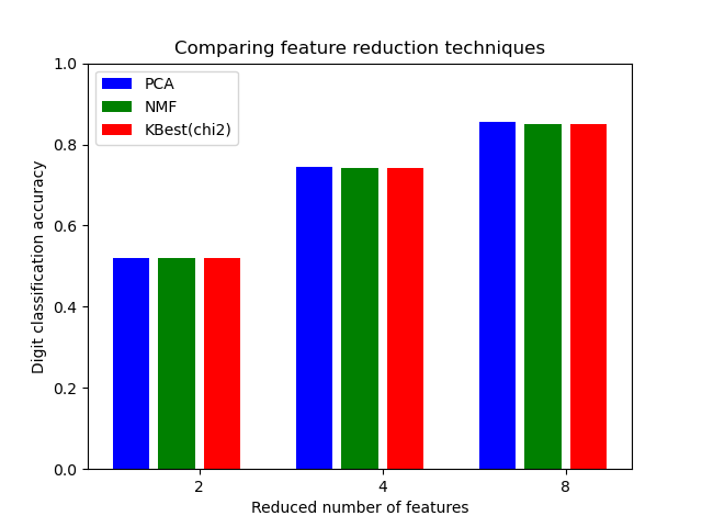
# Authors: Robert McGibbon, Joel Nothman, Guillaume Lemaitre


import numpy as np
import matplotlib.pyplot as plt
from sklearn.datasets import load_digits
from sklearn.model_selection import GridSearchCV
from sklearn.pipeline import Pipeline
from sklearn.svm import LinearSVC
from sklearn.decomposition import PCA, NMF
from sklearn.feature_selection import SelectKBest, chi2

print(__doc__)

pipe = Pipeline([
    # the reduce_dim stage is populated by the param_grid
    ('reduce_dim', 'passthrough'),
    ('classify', LinearSVC(dual=False, max_iter=10000))
])

N_FEATURES_OPTIONS = [2, 4, 8]
C_OPTIONS = [1, 10, 100, 1000]
param_grid = [
    {
        'reduce_dim': [PCA(iterated_power=7), NMF()],
        'reduce_dim__n_components': N_FEATURES_OPTIONS,
        'classify__C': C_OPTIONS
    },
    {
        'reduce_dim': [SelectKBest(chi2)],
        'reduce_dim__k': N_FEATURES_OPTIONS,
        'classify__C': C_OPTIONS
    },
]
reducer_labels = ['PCA', 'NMF', 'KBest(chi2)']

grid = GridSearchCV(pipe, n_jobs=1, param_grid=param_grid)
X, y = load_digits(return_X_y=True)
grid.fit(X, y)

mean_scores = np.array(grid.cv_results_['mean_test_score'])
# scores are in the order of param_grid iteration, which is alphabetical
mean_scores = mean_scores.reshape(len(C_OPTIONS), -1, len(N_FEATURES_OPTIONS))
# select score for best C
mean_scores = mean_scores.max(axis=0)
bar_offsets = (np.arange(len(N_FEATURES_OPTIONS)) *
               (len(reducer_labels) + 1) + .5)

plt.figure()
COLORS = 'bgrcmyk'
for i, (label, reducer_scores) in enumerate(zip(reducer_labels, mean_scores)):
    plt.bar(bar_offsets + i, reducer_scores, label=label, color=COLORS[i])

plt.title("Comparing feature reduction techniques")
plt.xlabel('Reduced number of features')
plt.xticks(bar_offsets + len(reducer_labels) / 2, N_FEATURES_OPTIONS)
plt.ylabel('Digit classification accuracy')
plt.ylim((0, 1))
plt.legend(loc='upper left')

plt.show()
Transforming target in regression
回归场景中 目标变量 需要转换的场景, 可以使用 TransformedTargetRegressor 工具。
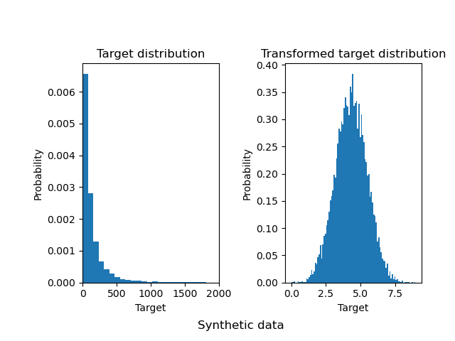
这种转换对外提供的数据输入和输出,都是原始数据。但是真正对于模型学习的目标是 经过转换器 正则化的数据。 正则化的数据具有更好的数据分布状态, 对于模型更加友好。
TransformedTargetRegressortransforms the targetsybefore fitting a regression model. The predictions are mapped back to the original space via an inverse transform. It takes as an argument the regressor that will be used for prediction, and the transformer that will be applied to the target variable:
例如 使用 QuantileTransformer 转换器,将倾斜的数据,转换为正态分布的数据。
>>> import numpy as np
>>> from sklearn.datasets import fetch_california_housing
>>> from sklearn.compose import TransformedTargetRegressor
>>> from sklearn.preprocessing import QuantileTransformer
>>> from sklearn.linear_model import LinearRegression
>>> from sklearn.model_selection import train_test_split
>>> X, y = fetch_california_housing(return_X_y=True)
>>> X, y = X[:2000, :], y[:2000]  # select a subset of data
>>> transformer = QuantileTransformer(output_distribution='normal')
>>> regressor = LinearRegression()
>>> regr = TransformedTargetRegressor(regressor=regressor,
...                                   transformer=transformer)
>>> X_train, X_test, y_train, y_test = train_test_split(X, y, random_state=0)
>>> regr.fit(X_train, y_train)
TransformedTargetRegressor(...)
>>> print('R2 score: {0:.2f}'.format(regr.score(X_test, y_test)))
R2 score: 0.61
>>> raw_target_regr = LinearRegression().fit(X_train, y_train)
>>> print('R2 score: {0:.2f}'.format(raw_target_regr.score(X_test, y_test)))
R2 score: 0.59
TransformedTargetRegressor
元估计器对于回归问题,应用于转换目标变量。
对于目标进行非线性变换, 例如 提供 QuantileTransformer, 或者提供 变换函数 和 逆变换函数。
Meta-estimator to regress on a transformed target.
Useful for applying a non-linear transformation to the target
yin regression problems. This transformation can be given as a Transformer such as the QuantileTransformer or as a function and its inverse such aslogandexp.The computation during
fitis:regressor.fit(X, func(y))or:
regressor.fit(X, transformer.transform(y))The computation during
predictis:inverse_func(regressor.predict(X))or:
transformer.inverse_transform(regressor.predict(X))Read more in the User Guide.
>>> import numpy as np
>>> from sklearn.linear_model import LinearRegression
>>> from sklearn.compose import TransformedTargetRegressor
>>> tt = TransformedTargetRegressor(regressor=LinearRegression(),
...                                 func=np.log, inverse_func=np.exp)
>>> X = np.arange(4).reshape(-1, 1)
>>> y = np.exp(2 * X).ravel()
>>> tt.fit(X, y)
TransformedTargetRegressor(...)
>>> tt.score(X, y)
1.0
>>> tt.regressor_.coef_
array([2.])
为什么要对目标进行变换?
https://scikit-learn.org/stable/auto_examples/compose/plot_transformed_target.html#sphx-glr-auto-examples-compose-plot-transformed-target-py
对于线性模型, 非均匀的数据蕴含的非线性特征,不容易抓取。
所以要讲数据进行均匀变换,或者正态变换。
In this example, we give an overview of
TransformedTargetRegressor. We use two examples to illustrate the benefit of transforming the targets before learning a linear regression model. The first example uses synthetic data while the second example is based on the Ames housing data set.
QuantileTransformer
使用百分位信息变换特征。
转换变量为均匀分布 或者 正态分布。
作用:
(1) 将稠密的分布展开。稠密分布就是最频繁的值。
(2)减少异常点的影响。
Transform features using quantiles information.
This method transforms the features to follow a uniform or a normal distribution. Therefore, for a given feature, this transformation tends to spread out the most frequent values. It also reduces the impact of (marginal) outliers: this is therefore a robust preprocessing scheme.
The transformation is applied on each feature independently. First an estimate of the cumulative distribution function of a feature is used to map the original values to a uniform distribution. The obtained values are then mapped to the desired output distribution using the associated quantile function. Features values of new/unseen data that fall below or above the fitted range will be mapped to the bounds of the output distribution. Note that this transform is non-linear. It may distort linear correlations between variables measured at the same scale but renders variables measured at different scales more directly comparable.
>>> import numpy as np
>>> from sklearn.preprocessing import QuantileTransformer
>>> rng = np.random.RandomState(0)
>>> X = np.sort(rng.normal(loc=0.5, scale=0.25, size=(25, 1)), axis=0)
>>> qt = QuantileTransformer(n_quantiles=10, random_state=0)
>>> qt.fit_transform(X)
array([...])
Compare the effect of different scalers on data with outliers -- 其它各种变换对异常点的影响
https://scikit-learn.org/stable/auto_examples/preprocessing/plot_all_scaling.html#sphx-glr-auto-examples-preprocessing-plot-all-scaling-py
FeatureUnion: composite feature spaces
特征联合,组合几个不同的特征变换对象, 成为一个新的变换对象, 并组合子变换输出。
对于数据特征的不同变换, 使用工具 ColumnTransformer。
特征联合 也是流水线的一部分,可以组件复杂的模型。
FeatureUnioncombines several transformer objects into a new transformer that combines their output. AFeatureUniontakes a list of transformer objects. During fitting, each of these is fit to the data independently. The transformers are applied in parallel, and the feature matrices they output are concatenated side-by-side into a larger matrix.When you want to apply different transformations to each field of the data, see the related class
ColumnTransformer(see user guide).
FeatureUnionserves the same purposes asPipeline- convenience and joint parameter estimation and validation.
FeatureUnionandPipelinecan be combined to create complex models.(A
FeatureUnionhas no way of checking whether two transformers might produce identical features. It only produces a union when the feature sets are disjoint, and making sure they are is the caller’s responsibility.)
两种特征变换输出的 特征值 组合 成一个新的特征向量。
A FeatureUnion is built using a list of (key, value) pairs, where the key is the name you want to give to a given transformation (an arbitrary string; it only serves as an identifier) and value is an estimator object:
>>>

>>> from sklearn.pipeline import FeatureUnion
>>> from sklearn.decomposition import PCA
>>> from sklearn.decomposition import KernelPCA
>>> estimators = [('linear_pca', PCA()), ('kernel_pca', KernelPCA())]
>>> combined = FeatureUnion(estimators)
>>> combined
FeatureUnion(transformer_list=[('linear_pca', PCA()),
                               ('kernel_pca', KernelPCA())])

Like pipelines, feature unions have a shorthand constructor called make_union that does not require explicit naming of the components.

Like Pipeline, individual steps may be replaced using set_params, and ignored by setting to 'drop':
>>>

>>> combined.set_params(kernel_pca='drop')
FeatureUnion(transformer_list=[('linear_pca', PCA()),
                               ('kernel_pca', 'drop')])
Concatenating multiple feature extraction methods --- feature union示例
https://scikit-learn.org/stable/auto_examples/compose/plot_feature_union.html#sphx-glr-auto-examples-compose-plot-feature-union-py
将PCA提取的特征 和 selectkbest提取的特征,组合为新的特征,送入svm模型。
In many real-world examples, there are many ways to extract features from a dataset. Often it is beneficial to combine several methods to obtain good performance. This example shows how to use
FeatureUnionto combine features obtained by PCA and univariate selection.Combining features using this transformer has the benefit that it allows cross validation and grid searches over the whole process.
The combination used in this example is not particularly helpful on this dataset and is only used to illustrate the usage of FeatureUnion.
Out:
Combined space has 3 features
Fitting 5 folds for each of 18 candidates, totalling 90 fits
[CV 1/5; 1/18] START features__pca__n_components=1, features__univ_select__k=1, svm__C=0.1
[CV 1/5; 1/18] END features__pca__n_components=1, features__univ_select__k=1, svm__C=0.1; total time=   0.0s
[CV 2/5; 1/18] START features__pca__n_components=1, features__univ_select__k=1, svm__C=0.1
[CV 2/5; 1/18] END features__pca__n_components=1, features__univ_select__k=1, svm__C=0.1; total time=   0.0s
[CV 3/5; 1/18] START features__pca__n_components=1, features__univ_select__k=1, svm__C=0.1
[CV 3/5; 1/18] END features__pca__n_components=1, features__univ_select__k=1, svm__C=0.1; total time=   0.0s
[CV 4/5; 1/18] START features__pca__n_components=1, features__univ_select__k=1, svm__C=0.1
[CV 4/5; 1/18] END features__pca__n_components=1, features__univ_select__k=1, svm__C=0.1; total time=   0.0s
[CV 5/5; 1/18] START features__pca__n_components=1, features__univ_select__k=1, svm__C=0.1
[CV 5/5; 1/18] END features__pca__n_components=1, features__univ_select__k=1, svm__C=0.1; total time=   0.0s
[CV 1/5; 2/18] START features__pca__n_components=1, features__univ_select__k=1, svm__C=1
[CV 1/5; 2/18] END features__pca__n_components=1, features__univ_select__k=1, svm__C=1; total time=   0.0s
[CV 2/5; 2/18] START features__pca__n_components=1, features__univ_select__k=1, svm__C=1
[CV 2/5; 2/18] END features__pca__n_components=1, features__univ_select__k=1, svm__C=1; total time=   0.0s
[CV 3/5; 2/18] START features__pca__n_components=1, features__univ_select__k=1, svm__C=1
[CV 3/5; 2/18] END features__pca__n_components=1, features__univ_select__k=1, svm__C=1; total time=   0.0s
[CV 4/5; 2/18] START features__pca__n_components=1, features__univ_select__k=1, svm__C=1
[CV 4/5; 2/18] END features__pca__n_components=1, features__univ_select__k=1, svm__C=1; total time=   0.0s
[CV 5/5; 2/18] START features__pca__n_components=1, features__univ_select__k=1, svm__C=1
[CV 5/5; 2/18] END features__pca__n_components=1, features__univ_select__k=1, svm__C=1; total time=   0.0s
[CV 1/5; 3/18] START features__pca__n_components=1, features__univ_select__k=1, svm__C=10
[CV 1/5; 3/18] END features__pca__n_components=1, features__univ_select__k=1, svm__C=10; total time=   0.0s
[CV 2/5; 3/18] START features__pca__n_components=1, features__univ_select__k=1, svm__C=10
[CV 2/5; 3/18] END features__pca__n_components=1, features__univ_select__k=1, svm__C=10; total time=   0.0s
[CV 3/5; 3/18] START features__pca__n_components=1, features__univ_select__k=1, svm__C=10
[CV 3/5; 3/18] END features__pca__n_components=1, features__univ_select__k=1, svm__C=10; total time=   0.0s
[CV 4/5; 3/18] START features__pca__n_components=1, features__univ_select__k=1, svm__C=10
[CV 4/5; 3/18] END features__pca__n_components=1, features__univ_select__k=1, svm__C=10; total time=   0.0s
[CV 5/5; 3/18] START features__pca__n_components=1, features__univ_select__k=1, svm__C=10
[CV 5/5; 3/18] END features__pca__n_components=1, features__univ_select__k=1, svm__C=10; total time=   0.0s
[CV 1/5; 4/18] START features__pca__n_components=1, features__univ_select__k=2, svm__C=0.1
[CV 1/5; 4/18] END features__pca__n_components=1, features__univ_select__k=2, svm__C=0.1; total time=   0.0s
[CV 2/5; 4/18] START features__pca__n_components=1, features__univ_select__k=2, svm__C=0.1
[CV 2/5; 4/18] END features__pca__n_components=1, features__univ_select__k=2, svm__C=0.1; total time=   0.0s
[CV 3/5; 4/18] START features__pca__n_components=1, features__univ_select__k=2, svm__C=0.1
[CV 3/5; 4/18] END features__pca__n_components=1, features__univ_select__k=2, svm__C=0.1; total time=   0.0s
[CV 4/5; 4/18] START features__pca__n_components=1, features__univ_select__k=2, svm__C=0.1
[CV 4/5; 4/18] END features__pca__n_components=1, features__univ_select__k=2, svm__C=0.1; total time=   0.0s
[CV 5/5; 4/18] START features__pca__n_components=1, features__univ_select__k=2, svm__C=0.1
[CV 5/5; 4/18] END features__pca__n_components=1, features__univ_select__k=2, svm__C=0.1; total time=   0.0s
[CV 1/5; 5/18] START features__pca__n_components=1, features__univ_select__k=2, svm__C=1
[CV 1/5; 5/18] END features__pca__n_components=1, features__univ_select__k=2, svm__C=1; total time=   0.0s
[CV 2/5; 5/18] START features__pca__n_components=1, features__univ_select__k=2, svm__C=1
[CV 2/5; 5/18] END features__pca__n_components=1, features__univ_select__k=2, svm__C=1; total time=   0.0s
[CV 3/5; 5/18] START features__pca__n_components=1, features__univ_select__k=2, svm__C=1
[CV 3/5; 5/18] END features__pca__n_components=1, features__univ_select__k=2, svm__C=1; total time=   0.0s
[CV 4/5; 5/18] START features__pca__n_components=1, features__univ_select__k=2, svm__C=1
[CV 4/5; 5/18] END features__pca__n_components=1, features__univ_select__k=2, svm__C=1; total time=   0.0s
[CV 5/5; 5/18] START features__pca__n_components=1, features__univ_select__k=2, svm__C=1
[CV 5/5; 5/18] END features__pca__n_components=1, features__univ_select__k=2, svm__C=1; total time=   0.0s
[CV 1/5; 6/18] START features__pca__n_components=1, features__univ_select__k=2, svm__C=10
[CV 1/5; 6/18] END features__pca__n_components=1, features__univ_select__k=2, svm__C=10; total time=   0.0s
[CV 2/5; 6/18] START features__pca__n_components=1, features__univ_select__k=2, svm__C=10
[CV 2/5; 6/18] END features__pca__n_components=1, features__univ_select__k=2, svm__C=10; total time=   0.0s
[CV 3/5; 6/18] START features__pca__n_components=1, features__univ_select__k=2, svm__C=10
[CV 3/5; 6/18] END features__pca__n_components=1, features__univ_select__k=2, svm__C=10; total time=   0.0s
[CV 4/5; 6/18] START features__pca__n_components=1, features__univ_select__k=2, svm__C=10
[CV 4/5; 6/18] END features__pca__n_components=1, features__univ_select__k=2, svm__C=10; total time=   0.0s
[CV 5/5; 6/18] START features__pca__n_components=1, features__univ_select__k=2, svm__C=10
[CV 5/5; 6/18] END features__pca__n_components=1, features__univ_select__k=2, svm__C=10; total time=   0.0s
[CV 1/5; 7/18] START features__pca__n_components=2, features__univ_select__k=1, svm__C=0.1
[CV 1/5; 7/18] END features__pca__n_components=2, features__univ_select__k=1, svm__C=0.1; total time=   0.0s
[CV 2/5; 7/18] START features__pca__n_components=2, features__univ_select__k=1, svm__C=0.1
[CV 2/5; 7/18] END features__pca__n_components=2, features__univ_select__k=1, svm__C=0.1; total time=   0.0s
[CV 3/5; 7/18] START features__pca__n_components=2, features__univ_select__k=1, svm__C=0.1
[CV 3/5; 7/18] END features__pca__n_components=2, features__univ_select__k=1, svm__C=0.1; total time=   0.0s
[CV 4/5; 7/18] START features__pca__n_components=2, features__univ_select__k=1, svm__C=0.1
[CV 4/5; 7/18] END features__pca__n_components=2, features__univ_select__k=1, svm__C=0.1; total time=   0.0s
[CV 5/5; 7/18] START features__pca__n_components=2, features__univ_select__k=1, svm__C=0.1
[CV 5/5; 7/18] END features__pca__n_components=2, features__univ_select__k=1, svm__C=0.1; total time=   0.0s
[CV 1/5; 8/18] START features__pca__n_components=2, features__univ_select__k=1, svm__C=1
[CV 1/5; 8/18] END features__pca__n_components=2, features__univ_select__k=1, svm__C=1; total time=   0.0s
[CV 2/5; 8/18] START features__pca__n_components=2, features__univ_select__k=1, svm__C=1
[CV 2/5; 8/18] END features__pca__n_components=2, features__univ_select__k=1, svm__C=1; total time=   0.0s
[CV 3/5; 8/18] START features__pca__n_components=2, features__univ_select__k=1, svm__C=1
[CV 3/5; 8/18] END features__pca__n_components=2, features__univ_select__k=1, svm__C=1; total time=   0.0s
[CV 4/5; 8/18] START features__pca__n_components=2, features__univ_select__k=1, svm__C=1
[CV 4/5; 8/18] END features__pca__n_components=2, features__univ_select__k=1, svm__C=1; total time=   0.0s
[CV 5/5; 8/18] START features__pca__n_components=2, features__univ_select__k=1, svm__C=1
[CV 5/5; 8/18] END features__pca__n_components=2, features__univ_select__k=1, svm__C=1; total time=   0.0s
[CV 1/5; 9/18] START features__pca__n_components=2, features__univ_select__k=1, svm__C=10
[CV 1/5; 9/18] END features__pca__n_components=2, features__univ_select__k=1, svm__C=10; total time=   0.0s
[CV 2/5; 9/18] START features__pca__n_components=2, features__univ_select__k=1, svm__C=10
[CV 2/5; 9/18] END features__pca__n_components=2, features__univ_select__k=1, svm__C=10; total time=   0.0s
[CV 3/5; 9/18] START features__pca__n_components=2, features__univ_select__k=1, svm__C=10
[CV 3/5; 9/18] END features__pca__n_components=2, features__univ_select__k=1, svm__C=10; total time=   0.0s
[CV 4/5; 9/18] START features__pca__n_components=2, features__univ_select__k=1, svm__C=10
[CV 4/5; 9/18] END features__pca__n_components=2, features__univ_select__k=1, svm__C=10; total time=   0.0s
[CV 5/5; 9/18] START features__pca__n_components=2, features__univ_select__k=1, svm__C=10
[CV 5/5; 9/18] END features__pca__n_components=2, features__univ_select__k=1, svm__C=10; total time=   0.0s
[CV 1/5; 10/18] START features__pca__n_components=2, features__univ_select__k=2, svm__C=0.1
[CV 1/5; 10/18] END features__pca__n_components=2, features__univ_select__k=2, svm__C=0.1; total time=   0.0s
[CV 2/5; 10/18] START features__pca__n_components=2, features__univ_select__k=2, svm__C=0.1
[CV 2/5; 10/18] END features__pca__n_components=2, features__univ_select__k=2, svm__C=0.1; total time=   0.0s
[CV 3/5; 10/18] START features__pca__n_components=2, features__univ_select__k=2, svm__C=0.1
[CV 3/5; 10/18] END features__pca__n_components=2, features__univ_select__k=2, svm__C=0.1; total time=   0.0s
[CV 4/5; 10/18] START features__pca__n_components=2, features__univ_select__k=2, svm__C=0.1
[CV 4/5; 10/18] END features__pca__n_components=2, features__univ_select__k=2, svm__C=0.1; total time=   0.0s
[CV 5/5; 10/18] START features__pca__n_components=2, features__univ_select__k=2, svm__C=0.1
[CV 5/5; 10/18] END features__pca__n_components=2, features__univ_select__k=2, svm__C=0.1; total time=   0.0s
[CV 1/5; 11/18] START features__pca__n_components=2, features__univ_select__k=2, svm__C=1
[CV 1/5; 11/18] END features__pca__n_components=2, features__univ_select__k=2, svm__C=1; total time=   0.0s
[CV 2/5; 11/18] START features__pca__n_components=2, features__univ_select__k=2, svm__C=1
[CV 2/5; 11/18] END features__pca__n_components=2, features__univ_select__k=2, svm__C=1; total time=   0.0s
[CV 3/5; 11/18] START features__pca__n_components=2, features__univ_select__k=2, svm__C=1
[CV 3/5; 11/18] END features__pca__n_components=2, features__univ_select__k=2, svm__C=1; total time=   0.0s
[CV 4/5; 11/18] START features__pca__n_components=2, features__univ_select__k=2, svm__C=1
[CV 4/5; 11/18] END features__pca__n_components=2, features__univ_select__k=2, svm__C=1; total time=   0.0s
[CV 5/5; 11/18] START features__pca__n_components=2, features__univ_select__k=2, svm__C=1
[CV 5/5; 11/18] END features__pca__n_components=2, features__univ_select__k=2, svm__C=1; total time=   0.0s
[CV 1/5; 12/18] START features__pca__n_components=2, features__univ_select__k=2, svm__C=10
[CV 1/5; 12/18] END features__pca__n_components=2, features__univ_select__k=2, svm__C=10; total time=   0.0s
[CV 2/5; 12/18] START features__pca__n_components=2, features__univ_select__k=2, svm__C=10
[CV 2/5; 12/18] END features__pca__n_components=2, features__univ_select__k=2, svm__C=10; total time=   0.0s
[CV 3/5; 12/18] START features__pca__n_components=2, features__univ_select__k=2, svm__C=10
[CV 3/5; 12/18] END features__pca__n_components=2, features__univ_select__k=2, svm__C=10; total time=   0.0s
[CV 4/5; 12/18] START features__pca__n_components=2, features__univ_select__k=2, svm__C=10
[CV 4/5; 12/18] END features__pca__n_components=2, features__univ_select__k=2, svm__C=10; total time=   0.0s
[CV 5/5; 12/18] START features__pca__n_components=2, features__univ_select__k=2, svm__C=10
[CV 5/5; 12/18] END features__pca__n_components=2, features__univ_select__k=2, svm__C=10; total time=   0.0s
[CV 1/5; 13/18] START features__pca__n_components=3, features__univ_select__k=1, svm__C=0.1
[CV 1/5; 13/18] END features__pca__n_components=3, features__univ_select__k=1, svm__C=0.1; total time=   0.0s
[CV 2/5; 13/18] START features__pca__n_components=3, features__univ_select__k=1, svm__C=0.1
[CV 2/5; 13/18] END features__pca__n_components=3, features__univ_select__k=1, svm__C=0.1; total time=   0.0s
[CV 3/5; 13/18] START features__pca__n_components=3, features__univ_select__k=1, svm__C=0.1
[CV 3/5; 13/18] END features__pca__n_components=3, features__univ_select__k=1, svm__C=0.1; total time=   0.0s
[CV 4/5; 13/18] START features__pca__n_components=3, features__univ_select__k=1, svm__C=0.1
[CV 4/5; 13/18] END features__pca__n_components=3, features__univ_select__k=1, svm__C=0.1; total time=   0.0s
[CV 5/5; 13/18] START features__pca__n_components=3, features__univ_select__k=1, svm__C=0.1
[CV 5/5; 13/18] END features__pca__n_components=3, features__univ_select__k=1, svm__C=0.1; total time=   0.0s
[CV 1/5; 14/18] START features__pca__n_components=3, features__univ_select__k=1, svm__C=1
[CV 1/5; 14/18] END features__pca__n_components=3, features__univ_select__k=1, svm__C=1; total time=   0.0s
[CV 2/5; 14/18] START features__pca__n_components=3, features__univ_select__k=1, svm__C=1
[CV 2/5; 14/18] END features__pca__n_components=3, features__univ_select__k=1, svm__C=1; total time=   0.0s
[CV 3/5; 14/18] START features__pca__n_components=3, features__univ_select__k=1, svm__C=1
[CV 3/5; 14/18] END features__pca__n_components=3, features__univ_select__k=1, svm__C=1; total time=   0.0s
[CV 4/5; 14/18] START features__pca__n_components=3, features__univ_select__k=1, svm__C=1
[CV 4/5; 14/18] END features__pca__n_components=3, features__univ_select__k=1, svm__C=1; total time=   0.0s
[CV 5/5; 14/18] START features__pca__n_components=3, features__univ_select__k=1, svm__C=1
[CV 5/5; 14/18] END features__pca__n_components=3, features__univ_select__k=1, svm__C=1; total time=   0.0s
[CV 1/5; 15/18] START features__pca__n_components=3, features__univ_select__k=1, svm__C=10
[CV 1/5; 15/18] END features__pca__n_components=3, features__univ_select__k=1, svm__C=10; total time=   0.0s
[CV 2/5; 15/18] START features__pca__n_components=3, features__univ_select__k=1, svm__C=10
[CV 2/5; 15/18] END features__pca__n_components=3, features__univ_select__k=1, svm__C=10; total time=   0.0s
[CV 3/5; 15/18] START features__pca__n_components=3, features__univ_select__k=1, svm__C=10
[CV 3/5; 15/18] END features__pca__n_components=3, features__univ_select__k=1, svm__C=10; total time=   0.0s
[CV 4/5; 15/18] START features__pca__n_components=3, features__univ_select__k=1, svm__C=10
[CV 4/5; 15/18] END features__pca__n_components=3, features__univ_select__k=1, svm__C=10; total time=   0.0s
[CV 5/5; 15/18] START features__pca__n_components=3, features__univ_select__k=1, svm__C=10
[CV 5/5; 15/18] END features__pca__n_components=3, features__univ_select__k=1, svm__C=10; total time=   0.0s
[CV 1/5; 16/18] START features__pca__n_components=3, features__univ_select__k=2, svm__C=0.1
[CV 1/5; 16/18] END features__pca__n_components=3, features__univ_select__k=2, svm__C=0.1; total time=   0.0s
[CV 2/5; 16/18] START features__pca__n_components=3, features__univ_select__k=2, svm__C=0.1
[CV 2/5; 16/18] END features__pca__n_components=3, features__univ_select__k=2, svm__C=0.1; total time=   0.0s
[CV 3/5; 16/18] START features__pca__n_components=3, features__univ_select__k=2, svm__C=0.1
[CV 3/5; 16/18] END features__pca__n_components=3, features__univ_select__k=2, svm__C=0.1; total time=   0.0s
[CV 4/5; 16/18] START features__pca__n_components=3, features__univ_select__k=2, svm__C=0.1
[CV 4/5; 16/18] END features__pca__n_components=3, features__univ_select__k=2, svm__C=0.1; total time=   0.0s
[CV 5/5; 16/18] START features__pca__n_components=3, features__univ_select__k=2, svm__C=0.1
[CV 5/5; 16/18] END features__pca__n_components=3, features__univ_select__k=2, svm__C=0.1; total time=   0.0s
[CV 1/5; 17/18] START features__pca__n_components=3, features__univ_select__k=2, svm__C=1
[CV 1/5; 17/18] END features__pca__n_components=3, features__univ_select__k=2, svm__C=1; total time=   0.0s
[CV 2/5; 17/18] START features__pca__n_components=3, features__univ_select__k=2, svm__C=1
[CV 2/5; 17/18] END features__pca__n_components=3, features__univ_select__k=2, svm__C=1; total time=   0.0s
[CV 3/5; 17/18] START features__pca__n_components=3, features__univ_select__k=2, svm__C=1
[CV 3/5; 17/18] END features__pca__n_components=3, features__univ_select__k=2, svm__C=1; total time=   0.0s
[CV 4/5; 17/18] START features__pca__n_components=3, features__univ_select__k=2, svm__C=1
[CV 4/5; 17/18] END features__pca__n_components=3, features__univ_select__k=2, svm__C=1; total time=   0.0s
[CV 5/5; 17/18] START features__pca__n_components=3, features__univ_select__k=2, svm__C=1
[CV 5/5; 17/18] END features__pca__n_components=3, features__univ_select__k=2, svm__C=1; total time=   0.0s
[CV 1/5; 18/18] START features__pca__n_components=3, features__univ_select__k=2, svm__C=10
[CV 1/5; 18/18] END features__pca__n_components=3, features__univ_select__k=2, svm__C=10; total time=   0.0s
[CV 2/5; 18/18] START features__pca__n_components=3, features__univ_select__k=2, svm__C=10
[CV 2/5; 18/18] END features__pca__n_components=3, features__univ_select__k=2, svm__C=10; total time=   0.0s
[CV 3/5; 18/18] START features__pca__n_components=3, features__univ_select__k=2, svm__C=10
[CV 3/5; 18/18] END features__pca__n_components=3, features__univ_select__k=2, svm__C=10; total time=   0.0s
[CV 4/5; 18/18] START features__pca__n_components=3, features__univ_select__k=2, svm__C=10
[CV 4/5; 18/18] END features__pca__n_components=3, features__univ_select__k=2, svm__C=10; total time=   0.0s
[CV 5/5; 18/18] START features__pca__n_components=3, features__univ_select__k=2, svm__C=10
[CV 5/5; 18/18] END features__pca__n_components=3, features__univ_select__k=2, svm__C=10; total time=   0.0s
Pipeline(steps=[('features',
                 FeatureUnion(transformer_list=[('pca', PCA(n_components=3)),
                                                ('univ_select',
                                                 SelectKBest(k=1))])),
                ('svm', SVC(C=10, kernel='linear'))])
# Author: Andreas Mueller <amueller@ais.uni-bonn.de>
#
# License: BSD 3 clause

from sklearn.pipeline import Pipeline, FeatureUnion
from sklearn.model_selection import GridSearchCV
from sklearn.svm import SVC
from sklearn.datasets import load_iris
from sklearn.decomposition import PCA
from sklearn.feature_selection import SelectKBest

iris = load_iris()

X, y = iris.data, iris.target

# This dataset is way too high-dimensional. Better do PCA:
pca = PCA(n_components=2)

# Maybe some original features were good, too?
selection = SelectKBest(k=1)

# Build estimator from PCA and Univariate selection:

combined_features = FeatureUnion([("pca", pca), ("univ_select", selection)])

# Use combined features to transform dataset:
X_features = combined_features.fit(X, y).transform(X)
print("Combined space has", X_features.shape[1], "features")

svm = SVC(kernel="linear")

# Do grid search over k, n_components and C:

pipeline = Pipeline([("features", combined_features), ("svm", svm)])

param_grid = dict(features__pca__n_components=[1, 2, 3],
                  features__univ_select__k=[1, 2],
                  svm__C=[0.1, 1, 10])

grid_search = GridSearchCV(pipeline, param_grid=param_grid, verbose=10)
grid_search.fit(X, y)
print(grid_search.best_estimator_)
ColumnTransformer
对异构数据的变换, 例如数值型 和 字符串型。
将特征提取和变换 组合成一个新的 变换。
Applies transformers to columns of an array or pandas DataFrame.
This estimator allows different columns or column subsets of the input to be transformed separately and the features generated by each transformer will be concatenated to form a single feature space. This is useful for heterogeneous or columnar data, to combine several feature extraction mechanisms or transformations into a single transformer.
对不同列的数据做不同正正则化, 并组装成新的特征向量。
>>> import numpy as np
>>> from sklearn.compose import ColumnTransformer
>>> from sklearn.preprocessing import Normalizer
>>> ct = ColumnTransformer(
...     [("norm1", Normalizer(norm='l1'), [0, 1]),
...      ("norm2", Normalizer(norm='l1'), slice(2, 4))])
>>> X = np.array([[0., 1., 2., 2.],
...               [1., 1., 0., 1.]])
>>> # Normalizer scales each row of X to unit norm. A separate scaling
>>> # is applied for the two first and two last elements of each
>>> # row independently.
>>> ct.fit_transform(X)
array([[0. , 1. , 0.5, 0.5],
       [0.5, 0.5, 0. , 1. ]])
ColumnTransformer for heterogeneous data
很多的数据集包含 不同类型的特征数据, 例如 文本, 浮点, 日期, 每种类型的特征,需要独立的预处理或者特征提取。
如果使用pandas处理出具,然后送入模型,这是有问题的:
(1)整合测试数据的统计特征,进入预处理器, 使得交叉验证的分值不稳定, 例如数据泄露。
(2)在参数搜索中,往往也希望能够搜索最优的变换参数。
Many datasets contain features of different types, say text, floats, and dates, where each type of feature requires separate preprocessing or feature extraction steps. Often it is easiest to preprocess data before applying scikit-learn methods, for example using pandas. Processing your data before passing it to scikit-learn might be problematic for one of the following reasons:
Incorporating statistics from test data into the preprocessors makes cross-validation scores unreliable (known as data leakage), for example in the case of scalers or imputing missing values.
You may want to include the parameters of the preprocessors in a parameter search.
The
ColumnTransformerhelps performing different transformations for different columns of the data, within aPipelinethat is safe from data leakage and that can be parametrized.ColumnTransformerworks on arrays, sparse matrices, and pandas DataFrames.
对于字符型数据使用 CountVectorizer 变换, 对于分类数据, 使用 OneHotEncoder 进行变换。
To each column, a different transformation can be applied, such as preprocessing or a specific feature extraction method:
>>> import pandas as pd
>>> X = pd.DataFrame(
...     {'city': ['London', 'London', 'Paris', 'Sallisaw'],
...      'title': ["His Last Bow", "How Watson Learned the Trick",
...                "A Moveable Feast", "The Grapes of Wrath"],
...      'expert_rating': [5, 3, 4, 5],
...      'user_rating': [4, 5, 4, 3]})
For this data, we might want to encode the
'city'column as a categorical variable usingOneHotEncoderbut apply aCountVectorizerto the'title'column. As we might use multiple feature extraction methods on the same column, we give each transformer a unique name, say'city_category'and'title_bow'. By default, the remaining rating columns are ignored (remainder='drop'):>>> from sklearn.compose import ColumnTransformer >>> from sklearn.feature_extraction.text import CountVectorizer >>> from sklearn.preprocessing import OneHotEncoder >>> column_trans = ColumnTransformer( ... [('city_category', OneHotEncoder(dtype='int'),['city']), ... ('title_bow', CountVectorizer(), 'title')], ... remainder='drop') >>> column_trans.fit(X) ColumnTransformer(transformers=[('city_category', OneHotEncoder(dtype='int'), ['city']), ('title_bow', CountVectorizer(), 'title')]) >>> column_trans.get_feature_names() ['city_category__x0_London', 'city_category__x0_Paris', 'city_category__x0_Sallisaw', 'title_bow__bow', 'title_bow__feast', 'title_bow__grapes', 'title_bow__his', 'title_bow__how', 'title_bow__last', 'title_bow__learned', 'title_bow__moveable', 'title_bow__of', 'title_bow__the', 'title_bow__trick', 'title_bow__watson', 'title_bow__wrath'] >>> column_trans.transform(X).toarray() array([[1, 0, 0, 1, 0, 0, 1, 0, 1, 0, 0, 0, 0, 0, 0, 0], [1, 0, 0, 0, 0, 0, 0, 1, 0, 1, 0, 0, 1, 1, 1, 0], [0, 1, 0, 0, 1, 0, 0, 0, 0, 0, 1, 0, 0, 0, 0, 0], [0, 0, 1, 0, 0, 1, 0, 0, 0, 0, 0, 1, 1, 0, 0, 1]]...)In the above example, the
CountVectorizerexpects a 1D array as input and therefore the columns were specified as a string ('title'). However,OneHotEncoderas most of other transformers expects 2D data, therefore in that case you need to specify the column as a list of strings (['city']).
通过 make_column_selector 定义 列的选择器, 这样不用显示指定列名。
Apart from a scalar or a single item list, the column selection can be specified as a list of multiple items, an integer array, a slice, a boolean mask, or with a
make_column_selector. Themake_column_selectoris used to select columns based on data type or column name:>>> from sklearn.preprocessing import StandardScaler >>> from sklearn.compose import make_column_selector >>> ct = ColumnTransformer([ ... ('scale', StandardScaler(), ... make_column_selector(dtype_include=np.number)), ... ('onehot', ... OneHotEncoder(), ... make_column_selector(pattern='city', dtype_include=object))]) >>> ct.fit_transform(X) array([[ 0.904..., 0. , 1. , 0. , 0. ], [-1.507..., 1.414..., 1. , 0. , 0. ], [-0.301..., 0. , 0. , 1. , 0. ], [ 0.904..., -1.414..., 0. , 0. , 1. ]])Strings can reference columns if the input is a DataFrame, integers are always interpreted as the positional columns.
Visualizing Composite Estimators
显示流水线结构图。
Estimators can be displayed with a HTML representation when shown in a jupyter notebook. This can be useful to diagnose or visualize a Pipeline with many estimators. This visualization is activated by setting the
displayoption inset_config:from sklearn import set_config set_config(display='diagram') # diplays HTML representation in a jupyter context column_trans