You can download this project from
https://github.com/lionzheng10/LaserMeasurement
The laser measurement project is come from Udacity Nano degree course "self driving car" term2, Lesson5.
Introduction
Imagine you are in a car equipped with sensors on the outside. The car sensors can detect objects moving around: for example, the sensors might detect a bicycle.
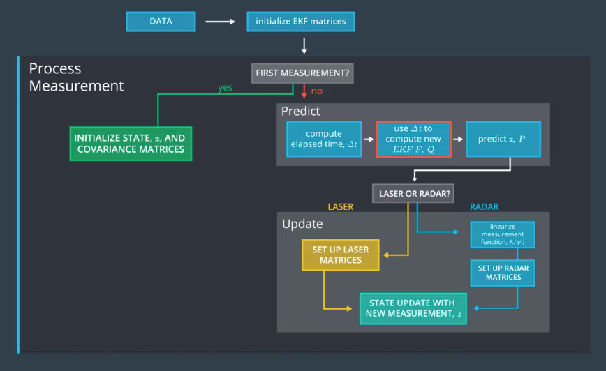
The Kalman Filter algorithm will go through the following steps:
- first measurement - the filter will receive initial measurements of the bicycle's position relative to the car. These measurements will come from a radar or lidar sensor.
- initialize state and covariance matrices - the filter will initialize the bicycle's position based on the first measurement.
- then the car will receive another sensor measurement after a time period Δt
- predict - the algorithm will predict where the bicycle will be after time Δt. One basic way to predict the bicycle location after Δt is to assume the bicycle's velocity is constant; thus the bicycle will have moved velocity * Δt. In the extended Kalman filter lesson, we will assume the velocity is constant; in the unscented Kalman filter lesson, we will introduce a more complex motion model.
- update - the filter compares the "predicted" location with what the sensor measurement says. The predicted location and the measured location are combined to give an updated location. The Kalman filter will put more weight on either the predicted location or the measured location depending on the uncertainty of each value.
- then the car will receive another sensor measurement after a time period Δt. The algorithm then does another predict and update step.
Kalman filter equation description
Kalman Filter overview
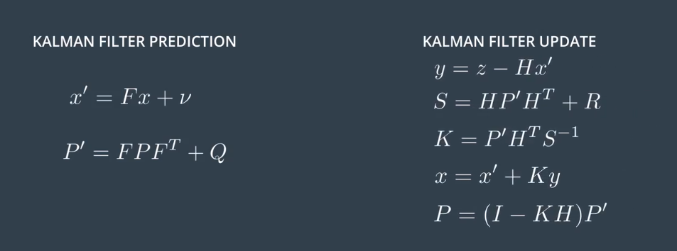

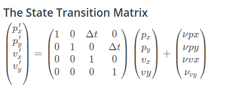
2D state motion. State transition matrix, x′ = Fx + v
- x is the mean state vector(4x1).For an extended Kalman filter, the mean state vector contains information about the object's position and velocity that you are tracking. It is called the "mean" state vector because position and velocity are represented by a gaussian distribution with mean x.
- v is a prediction noise (4x1)
- F is a state transition matrix (4 x 4), it's value is depend on Δt
- P is the state covariance matrix, which contains information about the uncertainty of the object's position and velocity.
- Q is process covariance matrix (4x4), see below
- z is the sensor information that tells where the object is relative to the car.
- y is difference between where we think we are with what the sensor tell us
y = z - Hx'. - H is a transform matrix. Depend on the shape of x and the shape of y, H is fixed matrix.
- R is the uncertainty of sensor measurement.
- S is the total uncertainty.
- K , often called Kalman filter gain, combines the uncertainty of where we think we are P' with the uncertainty of our sensor measurement R.
State transition Matrix F
Process Covariance Matrix Q
We need the process vovariance matrix to model the stochastic part of the state transition function.First I'm gosing to show you how the acceleration is expressed by the kinematic equations.And then I'm going to use that information to derive the process covariance matrix Q.

Say we have two consecutive observations of the same pedestrian with initial and final velocities. From the kinematic formulas we can derive the current position and speed as a function of previous state variables, including the change in the velocity or in other words, including the acceleration. You can see how this is derived below.
Looking at the deterministic part of our motion model, we assume the velocity is constant. However, in reality the pedestrian speed might change.Since the acceleration is unknown, we can add it to the noise component.And this random noise would be expressed analytically as in the last terms in the equation.
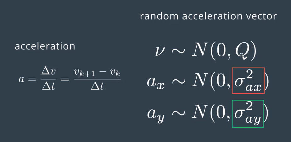
So, we have a random acceleration vector in this form, which is described by a 0 mean and the covariance matrix, Q. Delta t is computed at each Kalman filter step, and the acceleration is a random vector with 0 mean and standard deviations sigma ax and sigma ay.
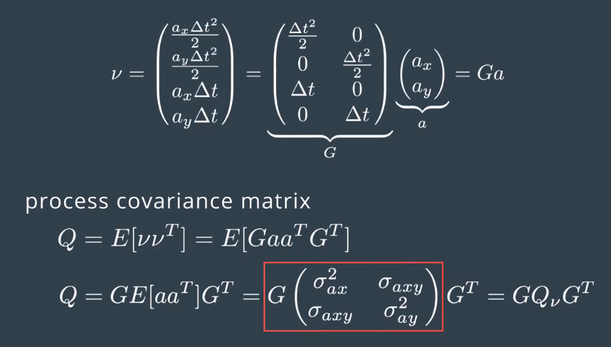
This vector can be decomposed into two components. A four by two matrix G which does not contain random variables. a, which contains the random acceleration components.
Based on our noise vector, we can define now the new covariance matrix Q. The covariance matrix is defined as the expectation value of the noise vector. mu times the noise vector mu transpose.So, let's write this down. As matrix G does not contain random variables, we can put it outside expectation calculation.
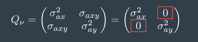
This leaves us with three statistical moments. The expectation of ax times ax, which is the variance of ax, sigma ax squared. The expectation if ay time ay which is the variance of ay, sigma ay squared. And the expectation of ax times ay which is the covariance of ax and ay. Ax and ay are assumed uncorrelated noise processes. This means that the covariace sigma ax, ay in Q nu is 0. So after combining everything in one matrix, we obtain our four by four Q matrix.
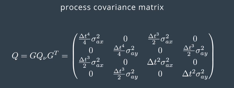
So after combining everything in one matrix, we obtain our four by four Q matrix.
Program structure
- main.cpp
The main.cpp readin the data file, extract data to a "Measurement package". Creat a tracking instance to analyze the data. - kalman_filter.h
DeclereKalmanFilterclass - kalman_filter.cpp
ImplementKalmanFilterfunctions,Predict()andUpdate() - tracking.h
Declare antrackingclass, it include anKalmanFilterinstance. - measurement_package.h
Define an classMeasurementPackageto store sensor type and measurement data. - tracking.cpp
The constructor functionTracking()declare the size and initial value ofKalman filtermatixes.
TheProcessMeasurementfunction process a single measurement, it compute the time elapsed between the current and previous measurements. Set the process covariance matrix Q. Call kalman filter functionpredictandupdate. And output state vector and Covariance Matrix. - obj_pose-laser-radar-synthetic-input.txt
A data file download from course web site, put it in the same folder with excutable file. - Eigen folder
Library for operate matix and vector and so on. Put this folder insrcfolder.
Makefile structure
- CMakeLists.txt
How to build and run this project
I am using ubuntu 16.4
- make sure you have cmake
sudo apt-get install camke - at the top level of the project repository
mkdir build && cd build - from /build
cmake .. && make - copy
obj_pose-laser-radar-synthetic-input.txttobuildfolder - from /build
./main
This is what the output looks like.
lion@HP6560b:~/carnd2/LaserMeasurement/build$ ./main
------ step0------
Kalman Filter Initialization

------ step1------
z_(lidar measure value: px,py)=
0.968521
 0.40545
x_(state vector: px,py,vx,vy)=
 0.96749
0.405862
 4.58427
-1.83232
P_(state Covariance Matrix)=
0.0224541         0  0.204131         0
        0 0.0224541         0  0.204131
 0.204131         0   92.7797         0
        0  0.204131         0   92.7797

------ step2------
z_(lidar measure value: px,py)=
0.947752
0.636824
x_(state vector: px,py,vx,vy)=
0.958365
0.627631
0.110368
 2.04304
P_(state Covariance Matrix)=
0.0220006         0  0.210519         0
        0 0.0220006         0  0.210519
 0.210519         0   4.08801         0
        0  0.210519         0   4.08801