Python中的Matplotlib绘图

Matplotlib 是一个 Python 的 2D绘图库，通过 Matplotlib，开发者可以仅需要几行代码，便可以生成绘图，直方图，功率谱，条形图，错误图，散点图等。

http://matplotlib.org

• 用于创建出版质量图表的绘图工具库

• 目的是为Python构建一个Matlab式的绘图接口

• import matplotlib.pyplot as plt

• pyploy模块包含了常用的matplotlib API函数

---

figure

• Matplotlib的图像均位于figure对象中

• 创建figure：fig = plt.figure()

# 引入matplotlib包
import matplotlib.pyplot as plt

# 创建figure对象
fig = plt.figure()

print(fig)

运行结果：

Figure(640x480)

设置图片大小

#设置图片大小
plt.figure(figsize=(20,8),dpi=80)

subplot

fig.add_subplot(a, b, c)

• a,b 表示将fig分割成 a*b 的区域

• c 表示当前选中要操作的区域，

• 注意：从1开始编号（不是从0开始）

• plot 绘图的区域是最后一次指定subplot的位置 (jupyter notebook里不能正确显示)

# 引入matplotlib包
import matplotlib.pyplot as plt
import numpy as np

# 创建figure对象
fig = plt.figure()
# 指定切分区域的位置
ax1 = fig.add_subplot(2, 2, 1)
ax2 = fig.add_subplot(2, 2, 2)
ax3 = fig.add_subplot(2, 2, 3)
ax4 = fig.add_subplot(2, 2, 4)

# 在subplot上作图
random_arr = np.random.randn(100)
# print random_arr

# 默认是在最后一次使用subplot的位置上作图，但是在jupyter notebook 里可能显示有误
plt.plot(random_arr)

# 可以指定在某个或多个subplot位置上作图
# ax1 = fig.plot(random_arr)
# ax2 = fig.plot(random_arr)
# ax3 = fig.plot(random_arr)

# 显示绘图结果
plt.show()

效果：

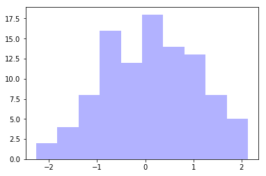
直方图：hist

import matplotlib.pyplot as plt
import numpy as np

plt.hist(np.random.randn(100), bins=10, color='b', alpha=0.3)
plt.show()

效果：

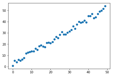
散点图：scatter

import matplotlib.pyplot as plt
import numpy as np

# 绘制散点图
x = np.arange(50)
y = x + 5 * np.random.rand(50)
plt.scatter(x, y)
plt.show()

效果：

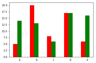
柱状图：bar

import matplotlib.pyplot as plt
import numpy as np

# 柱状图
x = np.arange(5)
y1, y2 = np.random.randint(1, 25, size=(2, 5))
width = 0.25
ax = plt.subplot(1,1,1)
ax.bar(x, y1, width, color='r')
ax.bar(x+width, y2, width, color='g')
ax.set_xticks(x+width)
ax.set_xticklabels(['a', 'b', 'c', 'd', 'e'])
plt.show()

效果：

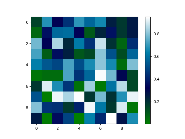
矩阵绘图：plt.imshow()

import matplotlib.pyplot as plt
import numpy as np

# 矩阵绘图
m = np.random.rand(10,10)
print(m)
plt.imshow(m, interpolation='nearest', cmap=plt.cm.ocean)
plt.colorbar()
plt.show()

效果：

[[0.15380616 0.67762688 0.31357941 0.44390774 0.68979664 0.57513838
  0.65629381 0.24503583 0.17923525 0.2571893 ]
 [0.06369402 0.36195036 0.58082668 0.58933892 0.32347774 0.09951149
  0.23330702 0.36485022 0.1841848  0.25991682]
 [0.7744867  0.31752527 0.84919452 0.22417739 0.62335052 0.44209677
  0.88063286 0.19690092 0.06757865 0.43073916]
 [0.72169407 0.09201384 0.35502444 0.24738157 0.10429607 0.14403884
  0.80343884 0.52208509 0.13111979 0.56812907]
 [0.63104273 0.53591166 0.49502278 0.72547993 0.51190937 0.66443688
  0.81036998 0.66157919 0.05206029 0.789589  ]
 [0.0310165  0.05378353 0.05515481 0.72832536 0.44728534 0.5773849
  0.94230944 0.7759232  0.30541425 0.14620932]
 [0.18399998 0.90858104 0.6671387  0.45428731 0.03820414 0.82961184
  0.02153911 0.60371894 0.86004263 0.14734495]
 [0.52464806 0.01133297 0.92722803 0.84628634 0.94730856 0.18697352
  0.78097648 0.19477215 0.67503973 0.92493486]
 [0.79691249 0.44451484 0.43481649 0.18034901 0.40381674 0.93531157
  0.61592443 0.18013501 0.90300771 0.02653334]
 [0.25387343 0.01286532 0.34527955 0.48654444 0.00421852 0.63679139
  0.41644148 0.95119758 0.27467997 0.66819625]]

 

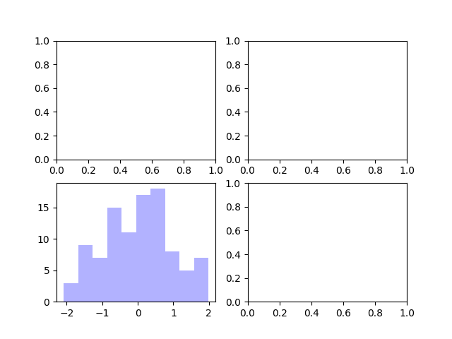
plt.subplots()

• 同时返回新创建的figure和subplot对象数组

• 生成2行2列subplot:fig, subplot_arr = plt.subplots(2,2)

• 在jupyter里可以正常显示，推荐使用这种方式创建多个图表

import matplotlib.pyplot as plt
import numpy as np

fig, subplot_arr = plt.subplots(2, 2)
# bins 为显示个数，一般小于等于数值个数
subplot_arr[1, 0].hist(np.random.randn(100), bins=10, color='b', alpha=0.3)
plt.savefig("./test.png")
plt.show()

效果：

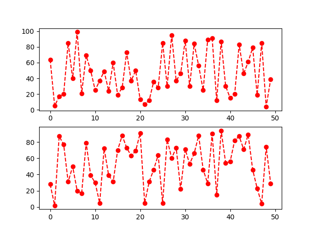
颜色、标记、线型

• ax.plot(x, y, ‘r--’)

等价于ax.plot(x, y, linestyle=‘--’, color=‘r’)

import matplotlib.pyplot as plt
import numpy as np

fig, axes = plt.subplots(2)
axes[0].plot(np.random.randint(0, 100, 50), 'ro--')
# 等价
axes[1].plot(np.random.randint(0, 100, 50), color='r', linestyle='dashed', marker='o')

效果：

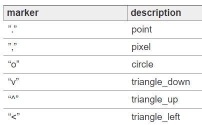
常用的颜色、标记、线型

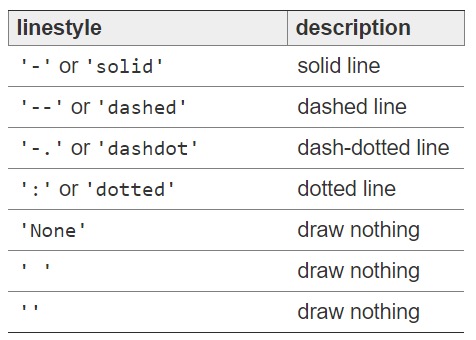
刻度、标签、图例

• 设置刻度范围

  plt.xlim(), plt.ylim()

  ax.set_xlim(), ax.set_ylim()

• 设置显示的刻度

  plt.xticks(), plt.yticks()

  ax.set_xticks(), ax.set_yticks()

• 设置刻度标签

  ax.set_xticklabels(), ax.set_yticklabels()

• 设置坐标轴标签

  ax.set_xlabel(), ax.set_ylabel()

• 设置标题

  ax.set_title()

• 图例

  ax.plot(label=‘legend’)

  ax.legend(), plt.legend()

  loc=‘best’：自动选择放置图例最佳位置

   

import matplotlib.pyplot as plt
import numpy as np

fig, ax = plt.subplots(1)
ax.plot(np.random.randn(1000).cumsum(), label='line0')

# 设置刻度
#plt.xlim([0,500])
ax.set_xlim([0, 800])

# 设置显示的刻度
#plt.xticks([0,500])
ax.set_xticks(range(0,500,100))

# 设置刻度标签
ax.set_yticklabels(['Jan', 'Feb', 'Mar'])

# 设置坐标轴标签
ax.set_xlabel('Number')
ax.set_ylabel('Month')

# 设置标题
ax.set_title('Example')

# 图例
ax.plot(np.random.randn(1000).cumsum(), label='line1')
ax.plot(np.random.randn(1000).cumsum(), label='line2')
ax.legend()
ax.legend(loc='best')
#plt.legend()
plt。show()

效果：

设置中文显示

为什么无法显示中文: matplotlib默认不支持中文字符，因为默认的英文字体无法显示汉字


查看linux/mac下面支持的字体:

fc-list   查看支持的字体

fc-list :lang=zh 查看支持的中文(冒号前面有空格)

如何修改matplotlib的默认字体?

        通过matplotlib.rc可以修改,具体方法参见源码(windows/linux)

        通过matplotlib 下的font_manager可以解决(windows/linux/mac)

# coding=utf-8
from matplotlib import pyplot as plt
import random
from matplotlib import font_manager

# windws和linux设置字体的放
# font = {'family' : 'MicroSoft YaHei',
#         'weight': 'bold',
#         'size': 'larger'}
# matplotlib.rc("font",**font)
# matplotlib.rc("font",family='MicroSoft YaHei',weight="bold")

# 另外一种设置字体的方式
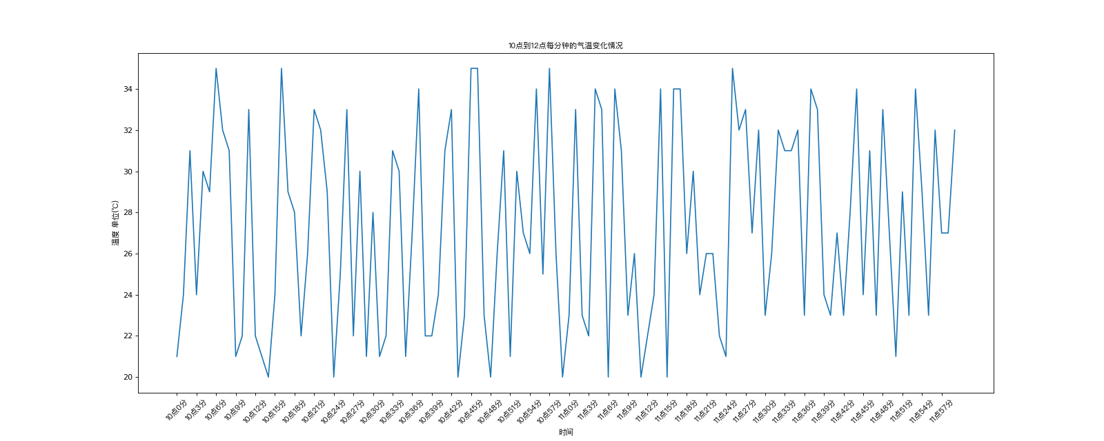
my_font = font_manager.FontProperties(fname="/System/Library/Fonts/PingFang.ttc")

x = range(0, 120)
y = [random.randint(20, 35) for i in range(120)]

plt.figure(figsize=(20, 8), dpi=80)

plt.plot(x, y)

# 调整x轴的刻度
_xtick_labels = ["10点{}分".format(i) for i in range(60)]
_xtick_labels += ["11点{}分".format(i) for i in range(60)]
# 取步长，数字和字符串一一对应，数据的长度一样
plt.xticks(list(x)[::3], _xtick_labels[::3], rotation=45, fontproperties=my_font)  # rotaion旋转的度数

# 添加描述信息
plt.xlabel("时间", fontproperties=my_font)
plt.ylabel("温度 单位(℃)", fontproperties=my_font)
plt.title("10点到12点每分钟的气温变化情况", fontproperties=my_font)

plt.show()

图片保存

#在plt.show()前面放置即可
plt.savefig("./picture.png") 

对比常用统计图总结：

折线图:以折线的上升或下降来表示统计数量的增减变化的统计图

特点:能够显示数据的变化趋势，反映事物的变化情况。(变化)

直方图:由一系列高度不等的纵向条纹或线段表示数据分布的情况。一般用横轴表示数据范围，纵轴表示分布情况。

特点:绘制连续性的数据,展示一组或者多组数据的分布状况(统计)

条形图:排列在工作表的列或行中的数据可以绘制到条形图中。

特点:绘制连离散的数据,能够一眼看出各个数据的大小,比较数据之间的差别。(统计)

散点图:用两组数据构成多个坐标点，考察坐标点的分布,判断两变量间是否存在某种关联或总结坐标点的分布模式。

特点:判断变量之间是否存在数量关联趋势,展示离群点(分布规律)

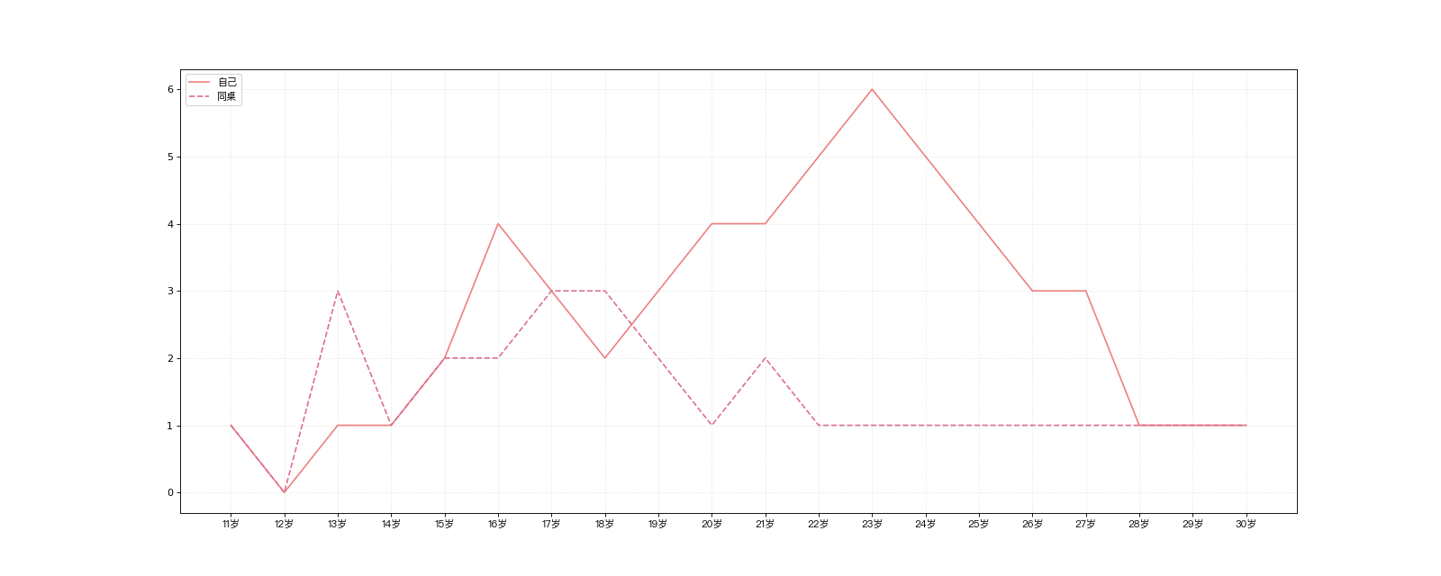
 示例demo

# coding=utf-8
from matplotlib import pyplot as plt
from matplotlib import font_manager

my_font = font_manager.FontProperties(fname="/System/Library/Fonts/PingFang.ttc")

y_1 = [1, 0, 1, 1, 2, 4, 3, 2, 3, 4, 4, 5, 6, 5, 4, 3, 3, 1, 1, 1]
y_2 = [1, 0, 3, 1, 2, 2, 3, 3, 2, 1, 2, 1, 1, 1, 1, 1, 1, 1, 1, 1]

x = range(11, 31)

# 设置图形大小
plt.figure(figsize=(20, 8), dpi=80)

plt.plot(x, y_1, label="自己", color="#F08080")
plt.plot(x, y_2, label="同桌", color="#DB7093", linestyle="--")

# 设置x轴刻度
_xtick_labels = ["{}岁".format(i) for i in x]
plt.xticks(x, _xtick_labels, fontproperties=my_font)
# plt.yticks(range(0,9))
# 绘制网格
plt.grid(alpha=0.4, linestyle=':')
# 添加图例
plt.legend(prop=my_font, loc="upper left")
# 保存
plt.savefig("./save.png")
#显示
plt.show()

效果：