4-支持向量机

理论部分

线性SVM分类

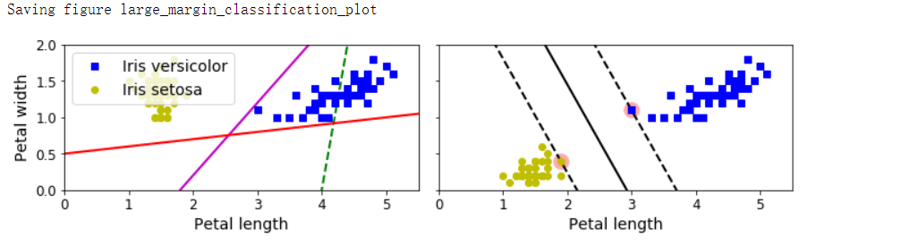
• 原理：可以将SVM分类器视为在类之间拟合可能的最宽的街道，因此也叫作最大间隔分类。在“街道以外”的地方增加更多训练实例不会对决策边界产生影响，也就是说它完全由位于街道边缘的实例所决定(或者称之为“支持”)，这些实例被称为支持向量
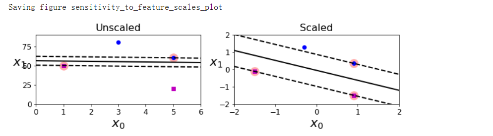
• SVM对特征的缩放非常敏感

软间隔分类

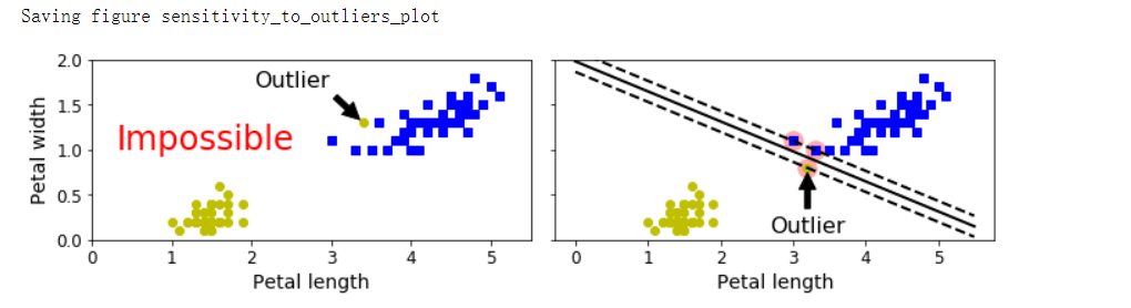
• 如果严格地让所有实例都不在街道上，并且位于正确的一边，这就是硬间隔分类；硬间隔分类有两个主要问题，首先，它只在数据是线性可分离的时候才有效；其次，它对异常值非常敏感
• 要避免这些问题，最好使用灵活的模型。目标是尽可能在保持街道宽阔和限制间隔违例之间找到良好的平衡，这就是软间隔分类

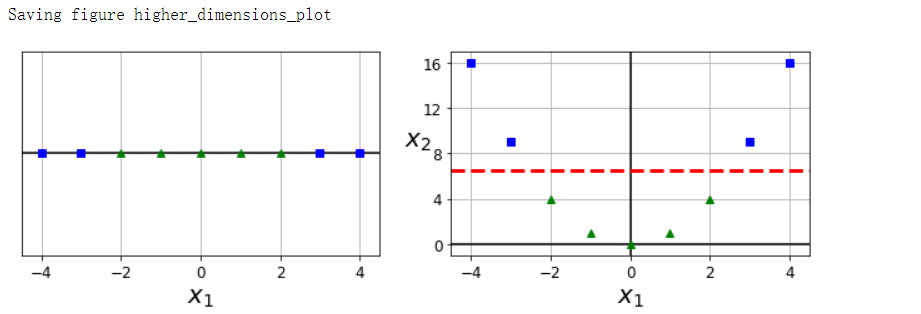
非线性SVM分类

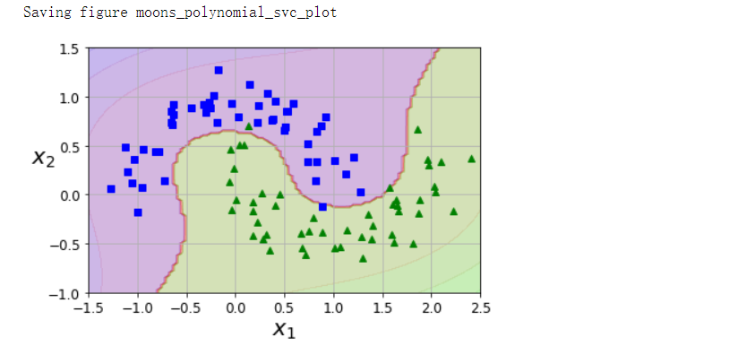
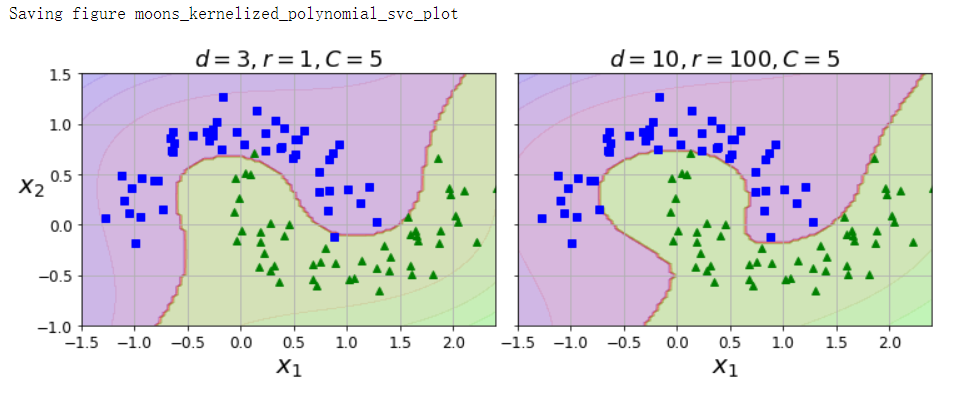
• 多项式内核
  • 使用SVM时，有一个魔术般的数学技巧可以应用，这就是核技巧。它产生的结果就跟添加了许多多项式特征(甚至是非常高阶的多项式特征)一样，但实际上并不需要真的添加。因为实际没有添加任何特征，所以也就不存在数量爆炸的组合特征了。

相似特征

• 解决非线性问题的另一种技术是添加相似特征，这些特征经过相似函数计算得出，相似函数可以测量每个实例与一个特定地标之间的相似度
• 原始不可分的数据集，经过相似函数转化后(去除了原始特征)可以呈现出线性可分的特性
• 如何选择地标：
  • 最简单的方法是在数据集里每一个实例的位置上创建一个地标。这会创造出许多维度，因而也增加了转换后的训练集线性可分离的机会
  • 缺点是如果训练集非常大，那就会得到同样大数量的特征

[高斯径向基函数(RBF)：phi_gamma(x, l) = exp(-gamma||x-l||^2) ]

高斯RBF核函数

• 高斯RBF核技巧产生的结果就跟添加了许多相似特征一样，但实际上也不需要添加
• 核函数选择
  • 有一个经验法则是：永远从线性核函数开始尝试，特别是训练集非常大或特征非常多的时候
  • 如果训练集不太大，你可以试试高斯RBF核，大多数情况下它都非常好用
  • 如果你还有多余的时间和计算能力，可以使用交叉验证和网格搜索来尝试一些其他的核函数，特别是那些专门针对你的数据集数据结构的核函数

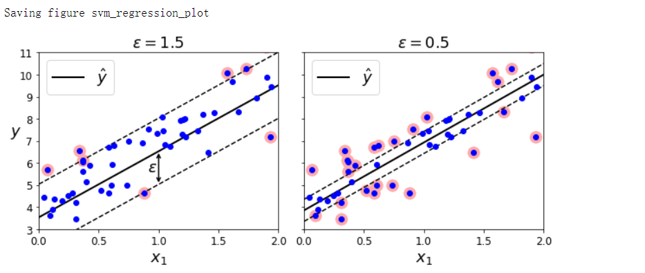
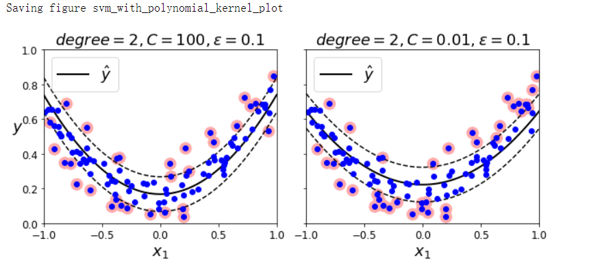
SVM回归

• SVM回归的目标：不再尝试拟合两个类之间可能的最宽街道的同时限制间隔违例，SVM回归要做的是让尽可能多的实例位于街道上，同时限制间隔违例(也就是不在街道上的实例)。
• 街道的宽度由ε控制，在间隔内添加更多的实例不会影响模型的预测，所以这个模型被称为ε不敏感
• 要解决非线性回归任务，可以使用核化的SVM回归模型

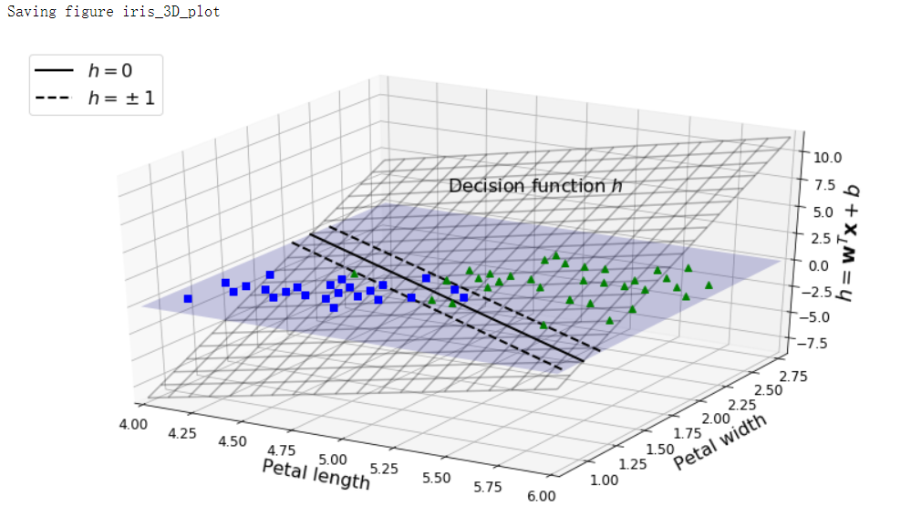
决策函数和预测

• 线性SVM分类器通过简单地计算决策函数w^Tx+b=w₁x₁+...+w_nx_n+b来预测新实例x的分类，如果结果为正，则预测类别是正类(1)，否则预测其为负类(0)

[hat y = left{ egin{matrix} -1， 如果w^Tx+b<0 \ 1，如果w^Tx+b >=0 end{matrix} ight . ]

训练目标

• 权重向量w越小，间隔越大，我们要最小化||w||来得到尽可能大的间隔
• 可以将硬间隔线性SVM分类器的目标看作一个约束优化问题

[minimizefrac{1}{2}w^Tw \ 使得t^{(i)}(w^Tx{(x)}+b)>=1,i=1, 2, ..., m ]

• 要达到软间隔的目标，需要为每个实例引入一个松弛变量ζ⁽ⁱ⁾>=0，ζ⁽ⁱ⁾衡量的是第i个实例多大程度上允许间隔违例。那么我们现在有两个互相冲突的目标：使松弛变量越小越好从而减少间隔违例，同时还要使w^Tw/2最小化以增大间隔

[软间隔线性SVM分类器目标：\ {underset {w,b,ζ} minimize}frac{1}{2}w^Tw + Csum^m_{i=1}ζ^{(i)} \ 使得t^{(i)}(w^Tx{(i)}+b)>=1-ζ^{(i)}和ζ^{(i)}>=0, i=1, 2, ..., m ]

二次规划

• 硬间隔和软间隔问题都属于线性约束的凸二次优化问题

[二次规划问题：\ {underset {p}minimize}frac{1}{2}p^THp+f^Tp，使得Ap<=b \ p是一个n_p维向量(n_p是参数向量) \ H是一个n_p*n_p的矩阵 \ f是一个n_p维的向量 \ A是一个n_c*n_p的矩阵(n_c是约束的数量) \ b是一个n_c维的向量 ]

• 不使用核技巧时可以用二次规划求解器求解

对偶问题

• 针对一个给定的约束优化问题，称之为原始问题，我们常常可以用另一个不同的，但是与之密切相关的问题来表达，这个问题我们称之为对偶问题。通常来说，对偶问题的解只能算是原始问题的解的下限，但是在某些情况下(目标函数是凸函数，不等式约束是连续可和凸函数)，它也可能跟原始问题的解完全相同，幸运的是，SVM问题刚好就满足这些条件

[线性SVM目标的对偶形式：\ {underset {alpha}minimize}frac{1}{2}sum^m_{i=1}sum^m_{j=1}alpha^{(i)}alpha^{(j)}t^{(i)}t^{(j)}x^{(i)T}x^{(j)}-sum^m_{i=1}alpha^{(i)} \ 使得alpha^{(i)}>=0,i=1, 2, ..., m ]

[一旦得到使得该等式最小化(使用二次规划求解器)的向量hatalpha，就可以使用下面的公式计算使原始问题最小化的hat w和hat b \ hat w = sum^m_{i=1}hat alpha ^{(i)}t^{(i)}x^{(i)} \ hat b = frac{1}{n_s}{underset {alpha^{(i)}>0} sum^m_{i=1}}(t^{(i)}-hat w^Tx^{(i)}) ]

• 当训练实例的数量小于特征数量时，解决对偶问题比原始问题更快速。更重要的是，它能够实现核技巧，而原始问题不可能实现

内核化SVM

• 转换后向量的点积等于原始向量点积的平方(二阶多项式映射的核技巧)

[phi(a)^Tphi(b)=(a^Tb)^2 \ 函数K(a, b)=(a^Tb)^2被称为二阶多项式核，在机器学习里，核是仅能够仅基于原始向量a和b来计算点积phi(a)^Tphi(b)的函数，\ 它不需要计算(甚至不需要知道)转换函数 ]

• 常用核函数

[线性：K(a, b)=a^Tb \ 多项式：K(a, b) = (gamma a^Tb+r)^d \ 高斯RBF：K(a, b) = exp(-gamma ||a-b||^2) \ Sigmoid：K(a, b) = tanh(gamma a^Tb+r) ]

[使用核化SVM做出预测：\ h_{hat w,hat b}(phi(x^{(n)})) = hat w^T phi(x^{(n)}) + hat b \ = (sum^m_{i=1}hat alpha^{(i)}t^{(i)}phi(x^{(i)}))^Tphi(x^{(n)})+hat b \ = sum^m_{i=1} hat alpha^{(i)}t^{(i)}(phi(x^{(i)}))^Tphi(x^{(n)})+hat b \ ={underset {hat alpha^{(i)}>0} sum^m_{i=1}}hat alpha^{(i=1)}t^{(i=1)}K(x^{(i)}, x^{(n)})+hat b ]

[使用核技巧来计算偏置项：\ hat b = frac{1}{n_s}{underset {hat alpha^{(i)}>0} sum^m_{i=1}}(t^{(i)}-hat w^Tphi(x^{(i)})) \ = frac{1}{n_s}{underset {hat alpha^{(i)}>0} sum^m_{i=1}}(t^{(i)}-(sum^m_{j=1}hat alpha^{(j)}t^{(i)}phi(x^{(j)}))^Tphi(x^{(i)})) \ = frac{1}{n_s}{underset {hat alpha^{(i)}>0} sum^m_{i=1}}(t^{(i)}-{underset {hat alpha^{(j)}>0} sum^m_{j=1}}hat alpha^{(j)}t^{(j)}K(x^{(i)}, x^{(j)})) ]

线性SVM分类器损失函数

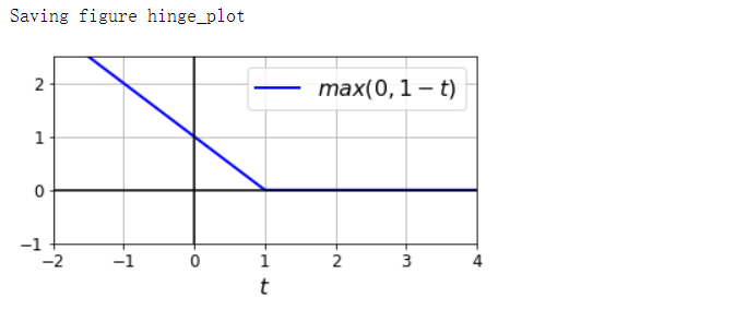
• 合页损失函数

  • 函数max(0, 1-t)被称为hinge损失函数。当t>=1时，函数等于0。如果t<1，其导数等于-1；如果t>1，则导数为0；t=1时，函数不可导。但是在t=0处可以使用任意次导数(即-1到0之间的任意值)，你还是可以使用梯度下降，就跟Lasso回归一样
  [线性SVM分类器成本函数：\ J(w, b)=frac{1}{2}w^Tw+Csum^m_{i=1}max(0, 1-t^{(i)}(w^Tx^{(i)}+b)) ]

代码部分

引入

import sys
assert sys.version_info >= (3, 5)

import sklearn
assert sklearn.__version__ >= '0.20'

import numpy as np
import os

np.random.seed(42)

%matplotlib inline
import matplotlib as mpl
import matplotlib.pyplot as plt
mpl.rc('axes', labelsize=14)
mpl.rc('xtick', labelsize=12)
mpl.rc('ytick', labelsize=12)

PROJECT_ROOT_DIR = '.'
CHAPTER_ID = 'svm'
IMAGES_PATH = os.path.join(PROJECT_ROOT_DIR, 'images', CHAPTER_ID)
os.makedirs(IMAGES_PATH, exist_ok=True)

def save_fig(fig_id, tight_layout=True, fig_extension='png', resolution=300):
    path = os.path.join(IMAGES_PATH, fig_id + '.' + fig_extension)
    print('Saving figure', fig_id)
    if tight_layout:
        plt.tight_layout()
    plt.savefig(path, format=fig_extension, dpi=resolution)

最大间隔分类

from sklearn.svm import SVC
from sklearn import datasets

iris = datasets.load_iris()
X = iris['data'][:, (2, 3)]
y = iris['target']

setosa_or_versicolor = (y == 0) | (y == 1)
X = X[setosa_or_versicolor]
y = y[setosa_or_versicolor]

svm_clf = SVC(kernel='linear', C=float('inf'))
svm_clf.fit(X, y)

# Bad models
x0 = np.linspace(0, 5.5, 200)
pred_1 = 5 * x0 - 20
pred_2 = x0 - 1.8
pred_3 = 0.1 * x0 + 0.5

def plot_svc_decision_boundary(svm_clf, xmin, xmax):
    w = svm_clf.coef_[0]
    b = svm_clf.intercept_[0]
    
    # 在决策边界，w0*x0 + w1*x1 + b = 0
    # => x1 = -w0/w1 * x0 - b/w1
    x0 = np.linspace(xmin, xmax, 200)
    decision_boundary = -w[0]/w[1] * x0 - b/w[1]
    
    margin = 1/w[1]
    gutter_up = decision_boundary + margin
    gutter_down = decision_boundary - margin
    
    svs = svm_clf.support_vectors_
    plt.scatter(svs[:, 0], svs[:, 1], s=180, facecolors='#FFAAAA')
    plt.plot(x0, decision_boundary, 'k-', linewidth=2)
    plt.plot(x0, gutter_up, 'k--', linewidth=2)
    plt.plot(x0, gutter_down, 'k--', linewidth=2)

fig, axes = plt.subplots(ncols=2, figsize=(10, 2.7), sharey=True)  # 同理，有：sharex
plt.sca(axes[0])
plt.plot(x0, pred_1, 'g--', linewidth=2)
plt.plot(x0, pred_2, 'm-', linewidth=2)
plt.plot(x0, pred_3, 'r-', linewidth=2)
plt.plot(X[:, 0][y==1], X[:, 1][y==1], 'bs', label='Iris versicolor')
plt.plot(X[:, 0][y==0], X[:, 1][y==1], 'yo', label='Iris setosa')
plt.xlabel('Petal length', fontsize=14)
plt.ylabel('Petal width', fontsize=14)
plt.legend(loc='upper left', fontsize=14)
plt.axis([0, 5.5, 0, 2])

plt.sca(axes[1])
plot_svc_decision_boundary(svm_clf, 0, 5.5)
plt.plot(X[:, 0][y==1], X[:, 1][y==1], 'bs')
plt.plot(X[:, 0][y==0], X[:, 1][y==0], 'yo')
plt.xlabel('Petal length', fontsize=14)
plt.axis([0, 5.5, 0, 2])

save_fig('large_margin_classification_plot')
plt.show()

特征缩放敏感

Xs = np.array([[1, 50], [5, 20], [3, 80], [5, 60]]).astype(np.float64)
ys = np.array([0, 0, 1, 1])
svm_clf = SVC(kernel='linear', C=100)
svm_clf.fit(Xs, ys)

plt.figure(figsize=(9, 2.7))
plt.subplot(121)
plt.plot(Xs[:, 0][ys==1], Xs[:, 1][ys==1], 'bo')
plt.plot(Xs[:, 0][ys==0], Xs[:, 1][ys==0], 'ms')
plot_svc_decision_boundary(svm_clf, 0, 6)
plt.xlabel('$x_0$', fontsize=20)
plt.ylabel('$x_1$', fontsize=20, rotation=0)
plt.title('Unscaled', fontsize=16)
plt.axis([0, 6, 0, 90])

from sklearn.preprocessing import StandardScaler

scaler = StandardScaler()
X_scaled = scaler.fit_transform(Xs)
svm_clf.fit(X_scaled, ys)

plt.subplot(122)
plt.plot(X_scaled[:, 0][ys==1], X_scaled[:, 1][ys==1], 'bo')
plt.plot(X_scaled[:, 0][ys==0], X_scaled[:, 1][ys==0], 'ms')
plot_svc_decision_boundary(svm_clf, -2, 2)
plt.xlabel('$x_0$', fontsize=20)
plt.ylabel('$x_1$', fontsize=20, rotation=0)
plt.title('Scaled', fontsize=16)
plt.axis([-2, 2, -2, 2])
save_fig('sensitivity_to_feature_scales_plot')

异常值敏感

X_outliers = np.array([[3.4, 1.3], [3.2, 0.8]])
y_outliers = np.array([0, 0])
Xo1 = np.concatenate([X, X_outliers[:1]], axis=0)
yo1 = np.concatenate([y, y_outliers[:1]], axis=0)
Xo2 = np.concatenate([X, X_outliers[1:]], axis=0)
yo2 = np.concatenate([y, y_outliers[1:]], axis=0)

svm_clf2 = SVC(kernel='linear', C=10**9)
svm_clf2.fit(Xo2, yo2)

fig, axes = plt.subplots(ncols=2, figsize=(10, 2.7), sharey=True)

plt.sca(axes[0])
plt.plot(Xo1[:, 0][yo1==1], Xo1[:, 1][yo1==1], 'bs')
plt.plot(Xo1[:, 0][yo1==0], Xo1[:, 1][yo1==0], 'yo')
plt.text(0.3, 1.0, 'Impossible', fontsize=24, color='red')
plt.xlabel('Petal length', fontsize=14)
plt.ylabel('Petal width', fontsize=14)
plt.annotate('Outlier', xy=(X_outliers[0][0], X_outliers[0][1]), xytext=(2.5, 1.7), 
             ha='center', arrowprops=dict(facecolor='black', shrink=0.1), fontsize=16)
plt.axis([0, 5.5, 0, 2])

plt.sca(axes[1])
plt.plot(Xo2[:, 0][yo2==1], Xo2[:, 1][yo2==1], 'bs')
plt.plot(Xo2[:, 0][yo2==0], Xo2[:, 1][yo2==0], 'yo')
plot_svc_decision_boundary(svm_clf2, 0, 5.5)
plt.xlabel('Petal length', fontsize=14)
plt.annotate('Outlier', xy=(X_outliers[1][0], X_outliers[1][1]), xytext=(3.2, 0.08), ha='center', 
            arrowprops=dict(facecolor='black', shrink=0.1), fontsize=16)
save_fig('sensitivity_to_outliers_plot')
plt.show()

通过调整C，调整间隔，达到正则化目的

import numpy as np
from sklearn import datasets
from sklearn.pipeline import Pipeline
from sklearn.preprocessing import StandardScaler
from sklearn.svm import LinearSVC

iris = datasets.load_iris()
X = iris['data'][:, (2, 3)]
y = (iris['target'] == 2).astype(np.float64)
svm_clf = Pipeline([
    ('scaler', StandardScaler()),
    ('linear_svc', LinearSVC(C=1, loss='hinge', random_state=42))
])
svm_clf.fit(X, y)

svm_clf.predict([[5.5, 1.7]])  # array([1.])

scaler = StandardScaler()
svm_clf1 = LinearSVC(C=1, loss='hinge', random_state=42)
svm_clf2 = LinearSVC(C=100, loss='hinge', random_state=42)

scaled_svm_clf1 = Pipeline([
    ('scaler', scaler), 
    ('linear_svc', svm_clf1),
])

scaled_svm_clf2 = Pipeline([
    ('scaler', scaler),
    ('linear_svc', svm_clf2),
])

scaled_svm_clf1.fit(X, y)
scaled_svm_clf2.fit(X, y)

# Convert to unscaled parameters
b1 = svm_clf1.decision_function([-scaler.mean_ / scaler.scale_])
b2 = svm_clf2.decision_function([-scaler.mean_ / scaler.scale_])
w1 = svm_clf1.coef_[0] / scaler.scale_
w2 = svm_clf2.coef_[0] / scaler.scale_
svm_clf1.intercept_ = np.array([b1])
svm_clf2.intercept_ = np.array([b2])
svm_clf1.coef_ = np.array([w1])
svm_clf2.coef_ = np.array([w2])
# Find support vectors (LinearSVC does not do this automatically)
t = y * 2 - 1
support_vectors_idx1 = (t * (X.dot(w1) + b1) < 1).ravel()
support_vectors_idx2 = (t * (X.dot(w2) + b2) < 1).ravel()
svm_clf1.support_vectors_ = X[support_vectors_idx1]
svm_clf2.support_vectors_ = X[support_vectors_idx2]

fig, axes = plt.subplots(ncols=2, figsize=(10, 2.7), sharey=True)
plt.sca(axes[0])
plt.plot(X[:, 0][y==1], X[:, 1][y==1], 'g^', label='Iris virginica')
plt.plot(X[:, 0][y==0], X[:, 1][y==0], 'bs', label='Iris versicolor')
plot_svc_decision_boundary(svm_clf1, 4, 5.9)
plt.xlabel('Petal length', fontsize=14)
plt.ylabel('Petal width', fontsize=14)
plt.legend(loc='upper left', fontsize=14)
plt.title('$C = {}$'.format(svm_clf1.C), fontsize=16)
plt.axis([4, 5.9, 0.8, 2.8])

plt.sca(axes[1])
plt.plot(X[:, 0][y==1], X[:, 1][y==1], 'g^')
plt.plot(X[:, 0][y==0], X[:, 1][y==0], 'bs')
plot_svc_decision_boundary(svm_clf2, 4, 5.99)
plt.xlabel('Petal length', fontsize=14)
plt.title('$C = {}$'.format(svm_clf2.C), fontsize=16)
plt.axis([4, 5.9, 0.8, 2.8])
save_fig('regularization_plot')

非线性分类

X1D = np.linspace(-4, 4, 9).reshape(-1, 1)
X2D = np.c_[X1D, X1D**2]
y = np.array([0, 0, 1, 1, 1, 1, 1, 0, 0])
plt.figure(figsize=(10, 3))
plt.subplot(121)
plt.grid(True, which='both')
plt.axhline(y=0, color='k')
plt.plot(X1D[:, 0][y==0], np.zeros(4), 'bs')
plt.plot(X1D[:, 0][y==1], np.zeros(5), 'g^')
plt.gca().get_yaxis().set_ticks([])
plt.xlabel(r'$x_1$', fontsize=20)
plt.axis([-4.5, 4.5, -0.2, 0.2])

plt.subplot(122)
plt.grid(True, which='both')
plt.axhline(y=0, color='k')
plt.axvline(x=0, color='k')
plt.plot(X2D[:, 0][y==0], X2D[:, 1][y==0], 'bs')
plt.plot(X2D[:, 0][y==1], X2D[:, 1][y==1], 'g^')
plt.xlabel(r'$x_1$', fontsize=20)
plt.ylabel(r'$x_2$', fontsize=20, rotation=0)
plt.gca().get_yaxis().set_ticks([0, 4, 8, 12, 16])
plt.plot([-4.5, 4.5], [6.5, 6.5], 'r--', linewidth=3)
plt.axis([-4.5, 4.5, -1, 17])
plt.subplots_adjust(right=1)
save_fig('higher_dimensions_plot', tight_layout=False)
plt.show()

from sklearn.datasets import make_moons

X, y = make_moons(n_samples=100, noise=0.15, random_state=42)

def plot_dataset(X, y, axes):
    plt.plot(X[:, 0][y==0], X[:, 1][y==0], 'bs')
    plt.plot(X[:, 0][y==1], X[:, 1][y==1], 'g^')
    plt.axis(axes)
    plt.grid(True, which='both')
    plt.xlabel(r'$x_1$', fontsize=20)
    plt.ylabel(r'$x_2$', fontsize=20, rotation=0)

plot_dataset(X, y, [-1.5, 2.5, -1, 1.5])
plt.show()

from sklearn.datasets import make_moons
from sklearn.pipeline import Pipeline
from sklearn.preprocessing import PolynomialFeatures

polynomial_svm_clf = Pipeline([
    ('poly_features', PolynomialFeatures(degree=3)),
    ('scaler', StandardScaler()),
    ('svm_clf', LinearSVC(C=10, loss='hinge', random_state=42)),
])
polynomial_svm_clf.fit(X, y)

def plot_predictions(clf, axes):
    x0s = np.linspace(axes[0], axes[1], 100)
    x1s = np.linspace(axes[2], axes[3], 100)
    x0, x1 = np.meshgrid(x0s, x1s)
    X = np.c_[x0.ravel(), x1.ravel()]
    y_pred = clf.predict(X).reshape(x0.shape)
    y_decision = clf.decision_function(X).reshape(x0.shape)
    plt.contourf(x0, x1, y_pred, cmap=plt.cm.brg, alpha=0.2)
    plt.contourf(x0, x1, y_decision, cmap=plt.cm.brg, alpha=0.1)

plot_predictions(polynomial_svm_clf, [-1.5, 2.5, -1, 1.5])
plot_dataset(X, y, [-1.5, 2.5, -1, 1.5])
save_fig('moons_polynomial_svc_plot')
plt.show()

多项式核

from sklearn.svm import SVC

poly_kernel_svm_clf = Pipeline([
    ('scaler', StandardScaler()),
    ('svm_clf', SVC(kernel='poly', degree=3, coef0=1, C=5))
])
poly_kernel_svm_clf.fit(X, y)

poly100_kernel_svm_clf = Pipeline([
    ('scaler', StandardScaler()),
    ('svm_clf', SVC(kernel='poly', degree=10, coef0=100, C=5))
])
poly100_kernel_svm_clf.fit(X, y)

fig, axes = plt.subplots(ncols=2, figsize=(10.5, 4), sharey=True)

plt.sca(axes[0])
plot_predictions(poly_kernel_svm_clf, [-1.5, 2.45, -1, 1.5])
plot_dataset(X, y, [-1.5, 2.4, -1, 1.5])
plt.title(r'$d=3, r=1, C=5$', fontsize=18)

plt.sca(axes[1])
plot_predictions(poly100_kernel_svm_clf, [-1.5, 2.4, -1, 1.5])
plot_dataset(X, y, [-1.5, 2.4, -1, 1.5])
plt.title(r'$d=10, r=100, C=5$', fontsize=18)
plt.ylabel('')

save_fig('moons_kernelized_polynomial_svc_plot')
plt.show()

高斯RBF核

def gaussian_rbf(x, landmark, gamma):
    return np.exp(-gamma * np.linalg.norm(x - landmark, axis=1) ** 2)

gamma = 0.3

x1s = np.linspace(-4.5, 4.5, 200).reshape(-1, 1)
x2s = gaussian_rbf(x1s, -2, gamma)
x3s = gaussian_rbf(x1s, 1, gamma)

XK = np.c_[gaussian_rbf(X1D, -2, gamma), gaussian_rbf(X1D, 1, gamma)]
yk = np.array([0, 0, 1, 1, 1, 1, 1, 0, 0])

plt.figure(figsize=(10.5, 4))
plt.subplot(121)
plt.grid(True, which='both')
plt.axhline(y=0, color='k')
plt.scatter(x=[-2, 1], y=[0, 0], s=150, alpha=0.5, c='red')
plt.plot(X1D[:, 0][yk==0], np.zeros(4), 'bs')
plt.plot(X1D[:, 0][yk==1], np.zeros(5), 'g^')
plt.plot(x1s, x2s, 'g--')
plt.plot(x1s, x3s, 'b:')
plt.gca().get_yaxis().set_ticks([0, 0.25, 0.5, 0.75, 1])
plt.xlabel(r'$x_1$', fontsize=20)
plt.ylabel(r'Similarity', fontsize=14)
plt.annotate(r'$mathbf{x}$', xy=(X1D[3, 0], 0), xytext=(-0.5, 0.20), ha='center', arrowprops=dict(facecolor='black', shrink=0.1), 
            fontsize=18)
plt.text(-2, 0.9, '$x_2$', ha='center', fontsize=20)
plt.text(1, 0.9, '$x_3$', ha='center', fontsize=20)
plt.axis([-4.5, 4.5, -0.1, 1.1])

plt.subplot(122)
plt.grid(True, which='both')
plt.axhline(y=0, color='k')
plt.axvline(x=0, color='k')
plt.plot(XK[:, 0][yk==0], XK[:, 1][yk==0], 'bs')
plt.plot(XK[:, 0][yk==1], XK[:, 1][yk==1], 'g^')
plt.xlabel(r'$x_2$', fontsize=20)
plt.ylabel(r'$x_3$', fontsize=20, rotation=0)
plt.annotate(r'$phileft(mathbf{x}
ight)$', xy=(XK[3, 0], XK[3, 1]), xytext=(0.65, 0.50), ha='center', 
            arrowprops=dict(facecolor='black', shrink=0.1), fontsize=18)
plt.plot([-0.1, 1.1], [0.57, -0.1], 'r--', linewidth=3)
plt.axis([-0.1, 1.1, -0.1, 1.1])
plt.subplots_adjust(right=1)
save_fig('kernel_method_plot')
plt.show()

x1_example = X1D[3, 0]
for landmark in (-2, 1):
    k = gaussian_rbf(np.array([[x1_example]]), np.array([[landmark]]), gamma)
    print('Phi({}, {}) = {}'.format(x1_example, landmark, k))

rbf_kernel_svm_clf = Pipeline([
    ('scaler', StandardScaler()),
    ('svm_clf', SVC(kernel='rbf', gamma=5, C=0.001))
])
rbf_kernel_svm_clf.fit(X, y)

from sklearn.svm import SVC

gamma1, gamma2 = 0.1, 5
C1, C2 = 0.001, 1000
hyperparams = (gamma1, C1), (gamma1, C2), (gamma2, C1), (gamma2, C2)

svm_clfs = []
for gamma, C in hyperparams:
    rbf_kernel_svm_clf = Pipeline([
        ('scaler', StandardScaler()),
        ('svm_clf', SVC(kernel='rbf', gamma=gamma, C=C))
    ])
    rbf_kernel_svm_clf.fit(X, y)
    svm_clfs.append(rbf_kernel_svm_clf)
fig, axes = plt.subplots(nrows=2, ncols=2, figsize=(10.5, 7), sharex=True, sharey=True)
for i, svm_clf in enumerate(svm_clfs):
    plt.sca(axes[i // 2, i % 2])
    plot_predictions(svm_clf, [-1.5, 2.45, -1, 1.5])
    plot_dataset(X, y, [-1.5, 2.45, -1, 1.5])
    gamma, C = hyperparams[i]
    plt.title(r'$gamma = {}, c= {}$'.format(gamma, C), fontsize=16)
    if i in (0, 1):
        plt.xlabel('')
    if i in (1, 3):
        plt.ylabel('')
save_fig('moons_rbf_svc_plot')
plt.show()

SVM回归

np.random.seed(42)
m = 50
X = 2 * np.random.rand(m, 1)
y = (4 + 3 * X + np.random.randn(m, 1)).ravel()

from sklearn.svm import LinearSVR

svm_reg = LinearSVR(epsilon=1.5, random_state=42)
svm_reg.fit(X, y)

svm_reg1 = LinearSVR(epsilon=1.5, random_state=42)
svm_reg2 = LinearSVR(epsilon=0.5, random_state=42)
svm_reg1.fit(X, y)
svm_reg2.fit(X, y)

def find_support_vectors(svm_reg, X, y):
    y_pred = svm_reg.predict(X)
    off_margin = (np.abs(y - y_pred) >= svm_reg.epsilon)
    return np.argwhere(off_margin)

svm_reg1.support_ = find_support_vectors(svm_reg1, X, y)
svm_reg2.support_ = find_support_vectors(svm_reg2, X, y)
eps_x1 = 1
eps_y_pred = svm_reg1.predict([[eps_x1]])

def plot_svm_regression(svm_reg, X, y, axes):
    x1s = np.linspace(axes[0], axes[1], 100).reshape(100, 1)
    y_pred = svm_reg.predict(x1s)
    plt.plot(x1s, y_pred, 'k-', linewidth=2, label=r'$hat{y}$')
    plt.plot(x1s, y_pred + svm_reg.epsilon, 'k--')
    plt.plot(x1s, y_pred - svm_reg.epsilon, 'k--')
    plt.scatter(X[svm_reg.support_], y[svm_reg.support_], s=180, facecolors='#FFAAAA')
    plt.plot(X, y, 'bo')
    plt.xlabel(r'$x_1$', fontsize=18)
    plt.legend(loc='upper left', fontsize=18)
    plt.axis(axes)

fig, axes = plt.subplots(ncols=2, figsize=(9, 4), sharey=True)
plt.sca(axes[0])
plot_svm_regression(svm_reg1, X, y, [0, 2, 3, 11])
plt.title(r'$epsilon = {}$'.format(svm_reg1.epsilon), fontsize=18)
plt.ylabel(r'$y$', fontsize=18, rotation=0)
plt.annotate('', xy=(eps_x1, eps_y_pred), xycoords='data', 
            xytext=(eps_x1, eps_y_pred - svm_reg1.epsilon), 
            textcoords='data', arrowprops={'arrowstyle': '<->', 'linewidth': 1.5})
plt.text(0.91, 5.6, r'$epsilon$'.format(svm_reg2.epsilon), fontsize=18)
plt.sca(axes[1])
plot_svm_regression(svm_reg2, X, y, [0, 2, 3, 11])
plt.title(r'$epsilon = {}$'.format(svm_reg2.epsilon), fontsize=18)
save_fig('svm_regression_plot')
plt.show()

SVM回归(利用核技巧)

np.random.seed(42)
m = 100
X = 2 * np.random.rand(m, 1) - 1
y = (0.2 + 0.1 * X + 0.5 * X ** 2 + np.random.randn(m, 1) / 10).ravel()

from sklearn.svm import SVR

svm_poly_reg = SVR(kernel='poly', degree=2, C=100, epsilon=0.1, gamma='scale')
svm_poly_reg.fit(X, y)

from sklearn.svm import SVR

svm_poly_reg1 = SVR(kernel='poly', degree=2, C=100, epsilon=0.1, gamma='scale')
svm_poly_reg2 = SVR(kernel='poly', degree=2, C=0.01, epsilon=0.1, gamma='scale')
svm_poly_reg1.fit(X, y)
svm_poly_reg2.fit(X, y)

fig, axes = plt.subplots(ncols=2, figsize=(9, 4), sharey=True)
plt.sca(axes[0])
plot_svm_regression(svm_poly_reg1, X, y, [-1, 1, 0, 1])
plt.title(r'$degree={}, C={}, epsilon={}$'.format(svm_poly_reg1.degree, 
                                                  svm_poly_reg1.C, 
                                                  svm_poly_reg1.epsilon), fontsize=18)
plt.ylabel(r'$y$', fontsize=18, rotation=0)
plt.sca(axes[1])
plot_svm_regression(svm_poly_reg2, X, y, [-1, 1, 0, 1])
plt.title(r'$degree={}, C={}, epsilon={}$'.format(svm_poly_reg2.degree, 
                                                  svm_poly_reg2.C, 
                                                  svm_poly_reg2.epsilon), fontsize=18)
save_fig('svm_with_polynomial_kernel_plot')
plt.show()

决策函数

iris = datasets.load_iris()
X = iris['data'][:, (2, 3)]
y = (iris['target'] == 2).astype(np.float64)

from mpl_toolkits.mplot3d import Axes3D

def plot_3D_decision_function(ax, w, b, x1_lim=[4, 6], x2_lim=[0.8, 2.8]):
    x1_in_bounds = (X[:, 0] > x1_lim[0]) & (X[:, 0] < x1_lim[1])
    X_crop = X[x1_in_bounds]
    y_crop = y[x1_in_bounds]
    x1s = np.linspace(x1_lim[0], x1_lim[1], 20)
    x2s = np.linspace(x2_lim[0], x2_lim[1], 20)
    x1, x2 = np.meshgrid(x1s, x2s)
    xs = np.c_[x1.ravel(), x2.ravel()]
    df = (xs.dot(w) + b).reshape(x1.shape)
    m = 1 / np.linalg.norm(w)
    boundary_x2s = -x1s*(w[0]/w[1])-b/w[1]
    margin_x2s_1 = -x1s*(w[0]/w[1])-(b-1)/w[1]
    margin_x2s_2 = -x1s*(w[0]/w[1])-(b+1)/w[1]
    ax.plot_surface(x1s, x2, np.zeros_like(x1),
                    color="b", alpha=0.2, cstride=100, rstride=100)
    ax.plot(x1s, boundary_x2s, 0, "k-", linewidth=2, label=r"$h=0$")
    ax.plot(x1s, margin_x2s_1, 0, "k--", linewidth=2, label=r"$h=pm 1$")
    ax.plot(x1s, margin_x2s_2, 0, "k--", linewidth=2)
    ax.plot(X_crop[:, 0][y_crop==1], X_crop[:, 1][y_crop==1], 0, "g^")
    ax.plot_wireframe(x1, x2, df, alpha=0.3, color="k")
    ax.plot(X_crop[:, 0][y_crop==0], X_crop[:, 1][y_crop==0], 0, "bs")
    ax.axis(x1_lim + x2_lim)
    ax.text(4.5, 2.5, 3.8, "Decision function $h$", fontsize=16)
    ax.set_xlabel(r"Petal length", fontsize=16, labelpad=10)
    ax.set_ylabel(r"Petal width", fontsize=16, labelpad=10)
    ax.set_zlabel(r"$h = mathbf{w}^T mathbf{x} + b$", fontsize=18, labelpad=5)
    ax.legend(loc="upper left", fontsize=16)

fig = plt.figure(figsize=(11, 6))
ax1 = fig.add_subplot(111, projection='3d')
plot_3D_decision_function(ax1, w=svm_clf2.coef_[0], b=svm_clf2.intercept_[0])

save_fig("iris_3D_plot")
plt.show()

训练目标

def plot_2D_decision_function(w, b, ylabel=True, x1_lim=[-3, 3]):
    x1 = np.linspace(x1_lim[0], x1_lim[1], 200)
    y = w * x1 + b
    m = 1 / w

    plt.plot(x1, y)
    plt.plot(x1_lim, [1, 1], "k:")
    plt.plot(x1_lim, [-1, -1], "k:")
    plt.axhline(y=0, color='k')
    plt.axvline(x=0, color='k')
    plt.plot([m, m], [0, 1], "k--")
    plt.plot([-m, -m], [0, -1], "k--")
    plt.plot([-m, m], [0, 0], "k-o", linewidth=3)
    plt.axis(x1_lim + [-2, 2])
    plt.xlabel(r"$x_1$", fontsize=16)
    if ylabel:
        plt.ylabel(r"$w_1 x_1$  ", rotation=0, fontsize=16)
    plt.title(r"$w_1 = {}$".format(w), fontsize=16)

fig, axes = plt.subplots(ncols=2, figsize=(9, 3.2), sharey=True)
plt.sca(axes[0])
plot_2D_decision_function(1, 0)
plt.sca(axes[1])
plot_2D_decision_function(0.5, 0, ylabel=False)
save_fig("small_w_large_margin_plot")
plt.show()

线性核

from sklearn.svm import SVC
from sklearn import datasets

iris = datasets.load_iris()
X = iris["data"][:, (2, 3)] # petal length, petal width
y = (iris["target"] == 2).astype(np.float64) # Iris virginica

svm_clf = SVC(kernel="linear", C=1)
svm_clf.fit(X, y)
svm_clf.predict([[5.3, 1.3]])

合页损失函数

t = np.linspace(-2, 4, 200)
h = np.where(1-t < 0, 0, 1-t)
plt.figure(figsize=(5, 2.8))
plt.plot(t, h, 'b-', linewidth=2, label='$max(0, 1-t)$')
plt.grid(True, which='both')
plt.axhline(y=0, color='k')
plt.axvline(x=0, color='k')
plt.yticks(np.arange(-1, 2.5, 1))
plt.xlabel('$t$', fontsize=16)
plt.axis([-2, 4, -1, 2.5])
plt.legend(loc='upper right', fontsize=16)
save_fig('hinge_plot')
plt.show()

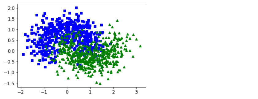
训练时间

from sklearn.datasets import make_moons

X, y = make_moons(n_samples=1000, noise=0.4, random_state=42)
plt.plot(X[:, 0][y==0], X[:, 1][y==0], 'bs')
plt.plot(X[:, 0][y==1], X[:, 1][y==1], 'g^')
plt.show()

import time
from sklearn.svm import SVC

tol = 0.1
tols = []
times = []
for i in range(10):
    svm_clf = SVC(kernel='poly', gamma=3, C=10, tol=tol, verbose=1)
    t1 = time.time()
    svm_clf.fit(X, y)
    t2 = time.time()
    tols.append(tol)
    times.append(t2-t1)
    print(i, tol, t2-t1)
    tol /= 10
# 此功能用于以x轴转换为对数格式的方式显示数据。当参数之一非常大并因此最初以紧凑方式存储时，此功能特别有用
# 这种轴半对数刻度曲线是将自变量对10取对数，可以有效的看出数据指数型变化时的衰变情况。
plt.semilogx(tols, times, 'bo-')
plt.xlabel('Tolerance', fontsize=16)
plt.ylabel('Time (seconds)', fontsize=16)
plt.grid(16)
plt.show()

使用批量梯度下降实现线性SVM

from sklearn.datasets import load_iris

iris = load_iris()
X = iris['data'][:, (2, 3)]
y = (iris['target'] == 2).astype(np.float64).reshape(-1, 1)

from sklearn.base import BaseEstimator

class MyLinearSVC(BaseEstimator):
    def __init__(self, C=1, eta0=1, eta_d=10000, n_epochs=1000, random_state=None):
        self.C = C
        self.eta0 = eta0
        self.n_epochs = n_epochs
        self.random_state = random_state
        self.eta_d = eta_d
    
    def eta(self, epoch):
        return self.eta0 / (epoch + self.eta_d)
    
    def fit(self, X, y):
        # Random initialization
        if self.random_state:
            np.random.seed(self.random_state)
        w = np.random.randn(X.shape[1], 1)
        b = 0
        m = len(X)
        t = y * 2 - 1  # -1 if y ==0, +1 if y==1
        X_t = X * t
        self.Js = []
        
        # Training
        for epoch in range(self.n_epochs):
            support_vectors_idx = (X_t.dot(w) + t * b < 1).ravel()
            X_t_sv = X_t[support_vectors_idx]
            t_sv = t[support_vectors_idx]
            J = 1/2 * np.sum(w * w) + self.C * (np.sum(1 - X_t_sv.dot(w)) - b * np.sum(t_sv))
            self.Js.append(J)
            w_gradient_vector = w - self.C * np.sum(X_t_sv, axis=0).reshape(-1, 1)
            b_derivative = -self.C * np.sum(t_sv)
            w = w - self.eta(epoch) * w_gradient_vector
            b = b - self.eta(epoch) * b_derivative
        self.intercept_ = np.array([b])
        self.coef_ = np.array([w])
        support_vectors_idx = (X_t.dot(w) + t * b < 1).ravel()
        self.support_vectors_ = X[support_vectors_idx]
        return self
    
    def decision_function(self, X):
        return X.dot(self.coef_[0]) + self.intercept_[0]
    
    def predict(self, X):
        return (self.decision_function(X) >= 0).astype(np.float64)
    

C = 2
svm_clf = MyLinearSVC(C=C, eta0=10, eta_d=1000, n_epochs=60000, random_state=42)
svm_clf.fit(X, y)
svm_clf.predict(np.array([[5, 2], [4, 1]]))  # array([[1.], [0.]])

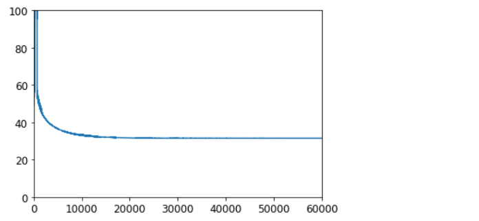
plt.plot(range(svm_clf.n_epochs), svm_clf.Js)
plt.axis([0, svm_clf.n_epochs, 0, 100])
plt.show()

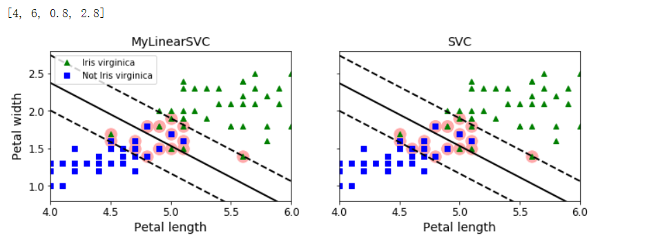
print(svm_clf.intercept_, svm_clf.coef_)  # [-15.56806513] [[[2.27960343] [2.7156819 ]]]

svm_clf2 = SVC(kernel='linear', C=C)
svm_clf2.fit(X, y.ravel())
print(svm_clf2.intercept_, svm_clf2.coef_)  # [-15.51721253] [[2.27128546 2.71287145]]

yr = y.ravel()
fig, axes = plt.subplots(ncols=2, figsize=(11, 3.2), sharey=True)
# 用于将当前轴设置为a
plt.sca(axes[0])
plt.plot(X[:, 0][yr==1], X[:, 1][yr==1], 'g^', label='Iris virginica')
plt.plot(X[:, 0][yr==0], X[:, 1][yr==0], 'bs', label='Not Iris virginica')
plot_svc_decision_boundary(svm_clf, 4, 6)
plt.xlabel('Petal length', fontsize=14)
plt.ylabel('Petal width', fontsize=14)
plt.title('MyLinearSVC', fontsize=14)
plt.axis([4, 6, 0.8, 2.8])
plt.legend(loc='upper left')

plt.sca(axes[1])
plt.plot(X[:, 0][yr==1], X[:, 1][yr==1], 'g^')
plt.plot(X[:, 0][yr==0], X[:, 1][yr==0], 'bs')
plot_svc_decision_boundary(svm_clf2, 4, 6)
plt.xlabel('Petal length', fontsize=14)
plt.title('SVC', fontsize=14)
plt.axis([4, 6, 0.8, 2.8])

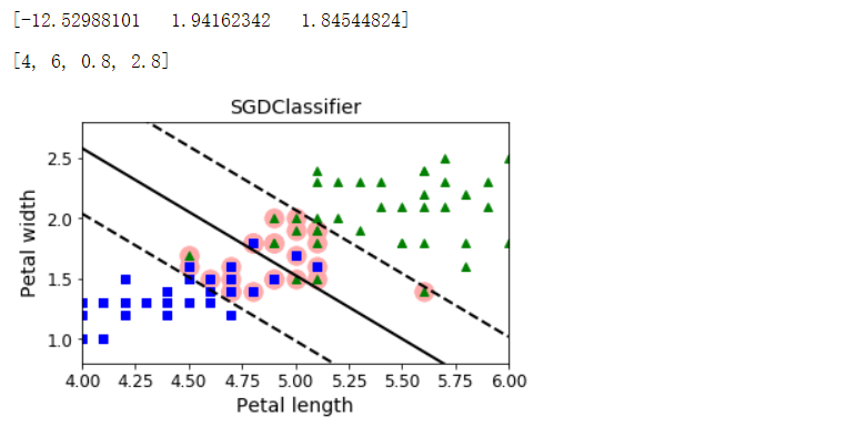
from sklearn.linear_model import SGDClassifier

sgd_clf = SGDClassifier(loss='hinge', alpha=0.017, max_iter=1000, tol=1e-3, random_state=42)
sgd_clf.fit(X, y.ravel())
m = len(X)
t = y * 2 - 1
X_b = np.c_[np.ones((m, 1)), X]  # Add bias input x0=1
X_b_t = X_b * t
# np.r_是按列连接两个矩阵，就是把两矩阵上下相加，要求列数相等，类似于pandas中的concat()
# np.c_是按行连接两个矩阵，就是把两矩阵左右相加，要求行数相等，类似于pandas中的merge()
sgd_theta = np.r_[sgd_clf.intercept_[0], sgd_clf.coef_[0]]
print(sgd_theta)
support_vectors_idx = (X_b_t.dot(sgd_theta) < 1).ravel()
sgd_clf.support_vectors_ = X[support_vectors_idx]
sgd_clf.C = C

plt.figure(figsize=(5.5, 3.2))
plt.plot(X[:, 0][yr==1], X[:, 1][yr==1], 'g^')
plt.plot(X[:, 0][yr==0], X[:, 1][yr==0], 'bs')
plot_svc_decision_boundary(sgd_clf, 4, 6)
plt.xlabel('Petal length', fontsize=14)
plt.ylabel('Petal width', fontsize=14)
plt.title('SGDClassifier', fontsize=14)
plt.axis([4, 6, 0.8, 2.8])