Numpy学习笔记（三）

有段时间没有写博客了，刚才看了看，上一篇写的时候还是在九月十四号，而现在已经是十月二十二号了。这段时间去哪里了？其实是去准备推免的复试。过程虽说有些艰辛，好在坚持了下来，最后是去了华东师范大学，地图学与地理信息系统的硕士，然后又在外面，一个人四处旅行，结实了三五好友，前几天才回来。回来既要准备科目二，又在学习HTML和CSS，Numpy的东西自然也不能落下。有一个感觉很明显：二十多天不碰，很多概念都已经生疏，再去接触，觉得很陌生。或许学习的状态就是如此，熟能生巧，用的少了，自然也就遗忘了。所以，还是得赶紧拾回来才行。

今天写的，是关于Numpy中的一些便捷函数，前面几次的练习也已经体会到内置函数的优越，这次会接触到更多。

Example1

股票相关性分析

# -*- coding:utf-8 -*-

import numpy as np

import matplotlib.pyplot as plt

 

#股票相关性分析

#提取数据

bhp = np.loadtxt("D:LearnCodepythonexerciseBHP.csv", delimiter=",", usecols=(6,), unpack=True)

bhp_returns = np.diff(bhp) / bhp[:-1]

 

vale = np.loadtxt("D:LearnCodepythonexerciseVALE.csv", delimiter=",", usecols=(6,), unpack=True)

vale_returns = np.diff(vale) / vale[:-1]

 

#计算协方差矩阵

covariance = np.cov(bhp_returns, vale_returns)

print "Covariance", covariance

 

#查看对角线元素

print "Covariance diagonal", covariance.diagonal()

 

# 计算迹

print "Covariance trace", covariance.trace()

 

#计算相关系数

print covariance / (bhp_returns.std()*vale_returns.std())

 

#下面的才是真正的相关系数矩阵

print "Covariance coefficient", np.corrcoef(bhp_returns, vale_returns)

 

# 判断走势是否同步

difference = bhp - vale

avg = np.mean(difference)

dev = np.std(difference)

# 判断最后一次交易是否同步

if np.abs(difference[-1]-avg) > 2*dev:

print "out of sync"

else:

print "in the sync"

 

# 绘图

t = np.arange(len(bhp_returns))

plt.plot(t, bhp_returns, lw=1.0)

plt.plot(t, vale_returns, lw=2.0)

plt.show()

结果如下：

Example2

多项式拟合

# 多项式拟合

bhp = np.loadtxt("D:LearnCodepythonexerciseBHP.csv", delimiter=",", usecols=(6, ), unpack=True)

vale = np.loadtxt("D:LearnCodepythonexerciseVALE.csv", delimiter=",", usecols=(6, ), unpack=True)

 

# 设置拟合次数

N = 3

 

# 调用拟合函数ployfit

t = np.arange(len(bhp))

poly = np.polyfit(t, bhp-vale, N)

print "Polynomial fit", poly

 

# 计算多项式函数的值

vals = np.polyval(poly, t)

 

# 判断下一个值

print "Next value", np.polyval(poly, t[-1]+1)

 

# 寻找零值

print "Roots", np.roots(poly)

 

# 求导

der = np.polyder(poly)

print "Derivative", der

 

# 导数的根即为函数的极值

print "Extremas", np.roots(der)

 

# 计算最大最小值

print "Max", np.argmax(vals)

print "Min", np.argmin(vals)

 

# 绘图

plt.plot(t, bhp-vale)

plt.plot(t, vals)

plt.show()

结果如下：

Example3

净额成交量

以某日为基期，逐日累计每日上市股票总成交量，若隔日指数或股票上涨，则基期OBV加上本日成交量为本日OBV，反之则相反。

# 净额成交量

c, v = np.loadtxt("D:LearnCodepythonexerciseBHP.csv", delimiter=",", usecols=(6, 7), unpack=True)

 

change = np.diff(c)

print "Change", change

 

#计算正负，两种方法

signs = np.sign(change)

print "Signs", signs

pieces = np.piecewise(change, [change < 0, change > 0], [-1, 1])

print "Pieces", pieces

# 检查两次输出是否一致

print "Array equal?", np.array_equal(signs, pieces)

 

# 计算OBV(净额成交量)

print "on balance volume", v[1:] * signs

结果如下：

Example4

交易过程模拟

# 交易过程模拟

o, h, l, c = np.loadtxt("D:LearnCodepythonexerciseBHP.csv", delimiter=",", usecols=(3, 4, 5, 6), unpack=True)

 

# 设置购买价与开盘价的比率

N = 0.99999

 

# 自定义一个相对利润函数

def calc_profit(open, high, low, close):

buy = open * N

if low < buy < high:

return (close-buy)/buy

else:

return 0

 

# 矢量化函数

func = np.vectorize(calc_profit)

profits = func(o, h, l, c)

 

print "Profits", profits

 

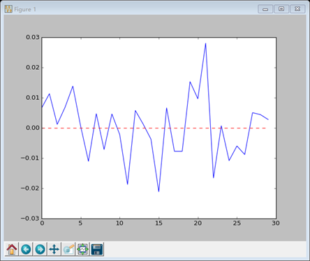
# 绘图

t = np.arange(len(o))

y = np.zeros(len(o))

plt.plot(t, profits)

plt.plot(t, y, 'r--')

plt.show()

 

# 计算交易的天数，并计算平均值

real_trades = profits[profits != 0]

print "Number of trades", len(real_trades), round(100*len(real_trades)/len(c), 2), '%'

print "Average profit/loss", round(100*np.mean(real_trades), 2), "%"

结果如下：

Example5

数据平滑

上一次用到了简单移动平均线对数据进行卷积运算，从而实现数据的平滑，这一次我们用Numpy内置的函数。

# 数据平滑

 

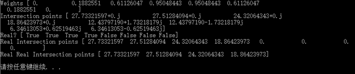
# 设置窗口的大小，并计算权重

N = 8

weights = np.hanning(N)

print "Weights", weights

 

# 卷积运算

bhp = np.loadtxt("D:LearnCodepythonexerciseBHP.csv", delimiter=",", usecols=(6, ), unpack=True)

bhp_returns = np.diff(bhp)/bhp[:-1]

smooth_bhp = np.convolve(weights/weights.sum(), bhp_returns)[N-1:-N+1]

vale = np.loadtxt("D:LearnCodepythonexerciseVALE.csv", delimiter=",", usecols=(6, ), unpack=True)

vale_returns = np.diff(vale)/vale[:-1]

smooth_vale = np.convolve(weights/weights.sum(), vale_returns)[N-1:-N+1]

 

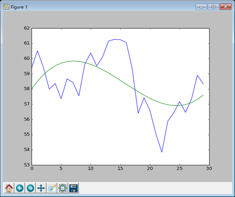
# 绘图

t = np.arange(N-1, len(bhp_returns))

plt.subplot(211)

plt.plot(t, bhp_returns[N-1:],'g--')

plt.plot(t, smooth_bhp,'g-',lw=2.0 )

plt.subplot(212)

plt.plot(t, vale_returns[N-1:], 'b--')

plt.plot(t, smooth_vale,'b-',lw=2.0 )

plt.show()

# 多项式拟合

K = 8 # 拟合次数

poly_bhp = np.polyfit(t, smooth_bhp, K)

poly_vale = np.polyfit(t, smooth_vale, K)

 

# 计算拟合函数交叉点

poly_sub = np.polysub(poly_bhp, poly_vale)

xpoints = np.roots(poly_sub)

print "Intersection points", xpoints

# 判断是否为实数

reals = np.isreal(xpoints)

print "Real?", reals

# select函数选择

xpoints = np.select([reals], [xpoints])

xpoints = xpoints.real

print "Real Intersection points", xpoints

 

# trim_zeros函数可以去掉一维数组中开头为0的元素

print "Real Real Intersection points", np.trim_zeros(xpoints)

结果如下：

 

总结：一段时间没有写，的确感觉很生疏，以前的一些基本概念也已经含混不清，还得是回过头去看，当然，学习的过程本就是这样，遗忘在所难免，这也就是我为什么倾向于迭代的学习，忘了的东西可以再去看，理解就是在这过程中慢慢深刻起来的。这一章的练习整体上不是很难，还是沿袭了Numpy的思路，熟练地使用是关键。

源代码：https://github.com/Lucifer25/Learn-Python/blob/master/Numpy/exercise3.py