zoukankan html css js c++ java

第14章循环神经网络

第14章循环神经网络

写在前面

参考书

《机器学习实战——基于Scikit-Learn和TensorFlow》

工具

python3.5.1，Jupyter Notebook, Pycharm

TensorFlow中的基本RNN

假设RNN只运行两个时间迭代，每个时间迭代输入一个大小为3的向量。

#!/usr/bin/env python
# -*- coding: UTF-8 -*-
# coding=utf-8 

"""
@author: Li Tian
@contact: 694317828@qq.com
@software: pycharm
@file: simple_rnn.py
@time: 2019/6/15 16:53
@desc: 实现一个最简单的RNN网络。我们将使用tanh激活函数创建一个由5个
        神经元组成的一层RNN。假设RNN只运行两个时间迭代，每个时间迭代
        输入一个大小为3的向量。
"""
import tensorflow as tf
import numpy as np

n_inputs = 3
n_neurons = 5

x0 = tf.placeholder(tf.float32, [None, n_inputs])
x1 = tf.placeholder(tf.float32, [None, n_inputs])

Wx = tf.Variable(tf.random_normal(shape=[n_inputs, n_neurons], dtype=tf.float32))
Wy = tf.Variable(tf.random_normal(shape=[n_neurons, n_neurons], dtype=tf.float32))
b = tf.Variable(tf.zeros([1, n_neurons], dtype=tf.float32))

y0 = tf.tanh(tf.matmul(x0, Wx) + b)
y1 = tf.tanh(tf.matmul(y0, Wy) + tf.matmul(x1, Wx) + b)

init = tf.global_variables_initializer()

# Mini-batch：包含4个实例的小批次
x0_batch = np.array([[0, 1, 2], [3, 4, 5], [6, 7, 8], [9, 0, 1]])   # t=0
x1_batch = np.array([[9, 8, 7], [0, 0, 0], [6, 5, 4], [3, 2, 1]])   # t=1

with tf.Session() as sess:
    init.run()
    y0_val, y1_val = sess.run([y0, y1], feed_dict={x0: x0_batch, x1: x1_batch})
    print(y0_val)
    print('-'*50)
    print(y1_val)

运行结果

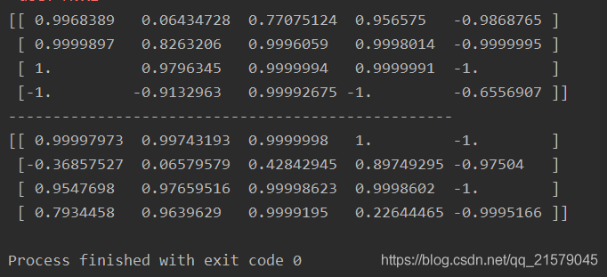
通过时间静态展开

static_rnn()函数通过链式单元来创建一个展开的RNN网络。

#!/usr/bin/env python
# -*- coding: UTF-8 -*-
# coding=utf-8 

"""
@author: Li Tian
@contact: 694317828@qq.com
@software: pycharm
@file: simple_rnn2.py
@time: 2019/6/15 17:06
@desc: 与前一个程序相同
"""

import tensorflow as tf
from tensorflow.contrib.rnn import BasicRNNCell
from tensorflow.contrib.rnn import static_rnn
import numpy as np

n_inputs = 3
n_neurons = 5

x0 = tf.placeholder(tf.float32, [None, n_inputs])
x1 = tf.placeholder(tf.float32, [None, n_inputs])

basic_cell = BasicRNNCell(num_units=n_neurons)
output_seqs, states = static_rnn(basic_cell, [x0, x1], dtype=tf.float32)

y0, y1 = output_seqs

init = tf.global_variables_initializer()

# Mini-batch：包含4个实例的小批次
x0_batch = np.array([[0, 1, 2], [3, 4, 5], [6, 7, 8], [9, 0, 1]])   # t=0
x1_batch = np.array([[9, 8, 7], [0, 0, 0], [6, 5, 4], [3, 2, 1]])   # t=1

with tf.Session() as sess:
    init.run()
    y0_val, y1_val = sess.run([y0, y1], feed_dict={x0: x0_batch, x1: x1_batch})
    print(y0_val)
    print('-'*50)
    print(y1_val)

运行结果

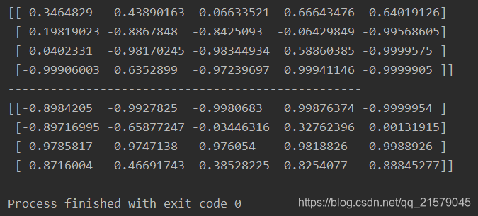
通过时间动态展开

利用dynamic_rnn()和while_loop()

#!/usr/bin/env python
# -*- coding: UTF-8 -*-
# coding=utf-8 

"""
@author: Li Tian
@contact: 694317828@qq.com
@software: pycharm
@file: dynamic_rnn1.py
@time: 2019/6/16 13:37
@desc:  通过时间动态展开 dynamic_rnn
"""

import tensorflow as tf
from tensorflow.contrib.rnn import BasicRNNCell
import numpy as np


n_steps = 2
n_inputs = 3
n_neurons = 5

x = tf.placeholder(tf.float32, [None, n_steps, n_inputs])
basic_cell = BasicRNNCell(num_units=n_neurons)
outputs, states = tf.nn.dynamic_rnn(basic_cell, x, dtype=tf.float32)

x_batch = np.array([
    [[0, 1, 2], [9, 8, 7]],
    [[3, 4, 5], [0, 0, 0]],
    [[6, 7, 8], [6, 5, 4]],
    [[9, 0, 1], [3, 2, 1]],
])

init = tf.global_variables_initializer()

with tf.Session() as sess:
    init.run()
    outputs_val = outputs.eval(feed_dict={x: x_batch})
    print(outputs_val)

运行结果

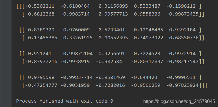
这时问题来了，动态、静态这两种有啥区别呢？

参考：tensor flow dynamic_rnn 与rnn有啥区别？

处理长度可变输入序列

#!/usr/bin/env python
# -*- coding: UTF-8 -*-
# coding=utf-8 

"""
@author: Li Tian
@contact: 694317828@qq.com
@software: pycharm
@file: dynamic_rnn2.py
@time: 2019/6/17 9:42
@desc: 处理长度可变输入序列
"""

import tensorflow as tf
from tensorflow.contrib.rnn import BasicRNNCell
import numpy as np


n_steps = 2
n_inputs = 3
n_neurons = 5

seq_length = tf.placeholder(tf.int32, [None])
x = tf.placeholder(tf.float32, [None, n_steps, n_inputs])
basic_cell = BasicRNNCell(num_units=n_neurons)
outputs, states = tf.nn.dynamic_rnn(basic_cell, x, dtype=tf.float32, sequence_length=seq_length)

# 假设第二个输出序列仅包含一个输入。为了适应输入张量X，必须使用零向量填充输入。
x_batch = np.array([
    [[0, 1, 2], [9, 8, 7]],
    [[3, 4, 5], [0, 0, 0]],
    [[6, 7, 8], [6, 5, 4]],
    [[9, 0, 1], [3, 2, 1]],
])

seq_length_batch = np.array([2, 1, 2, 2])

init = tf.global_variables_initializer()

with tf.Session() as sess:
    init.run()
    outputs_val, states_val = sess.run([outputs, states], feed_dict={x: x_batch, seq_length: seq_length_batch})
    print(outputs_val)

运行结果

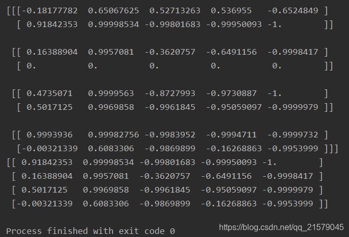
结果分析

RNN每一次迭代超过输入长度的部分输出零向量。

此外，状态张量包含了每个单元的最终状态（除了零向量）。

处理长度可变输出序列

最通常的解决方案是定义一种被称为序列结束令牌（EOS token）的特殊输出。

训练RNN

通过时间反向传播（BPTT）：梯度通过被成本函数使用的所有输出向后流动，而不是仅仅通过输出最终输出。

训练序列分类器

#!/usr/bin/env python
# -*- coding: UTF-8 -*-
# coding=utf-8 

"""
@author: Li Tian
@contact: 694317828@qq.com
@software: pycharm
@file: rnn_test1.py
@time: 2019/6/17 10:28
@desc: 训练一个识别MNIST图像的RNN网络。
"""

import tensorflow as tf
from tensorflow.contrib.layers import fully_connected
from tensorflow.contrib.rnn import BasicRNNCell

from tensorflow.examples.tutorials.mnist import input_data


n_steps = 28
n_inputs = 28
n_neurons = 150
n_outputs = 10

learning_rate = 0.001

n_epochs = 100
batch_size = 150

X = tf.placeholder(tf.float32, [None, n_steps, n_inputs])
y = tf.placeholder(tf.int32, [None])

basic_cell = BasicRNNCell(num_units=n_neurons)
outputs, states = tf.nn.dynamic_rnn(basic_cell, X, dtype=tf.float32)

logits = fully_connected(states, n_outputs, activation_fn=None)
xentropy = tf.nn.sparse_softmax_cross_entropy_with_logits(labels=y, logits=logits)

loss = tf.reduce_mean(xentropy)
optimizer = tf.train.AdamOptimizer(learning_rate=learning_rate)
training_op = optimizer.minimize(loss)
correct = tf.nn.in_top_k(logits, y, 1)
accuracy = tf.reduce_mean(tf.cast(correct, tf.float32))
init = tf.global_variables_initializer()

# 加载MNIST数据，并按照网格的要求改造测试数据。
mnist = input_data.read_data_sets('D:/Python3Space/BookStudy/book2/MNIST_data/')
X_test = mnist.test.images.reshape((-1, n_steps, n_inputs))
y_test = mnist.test.labels

with tf.Session() as sess:
    init.run()
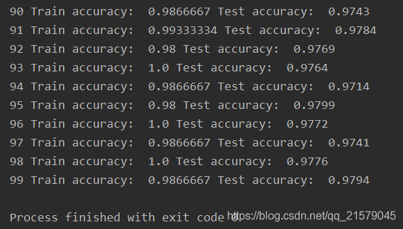
    for epoch in range(n_epochs):
        for iteration in range(mnist.train.num_examples // batch_size):
            X_batch, y_batch = mnist.train.next_batch(batch_size)
            X_batch = X_batch.reshape((-1, n_steps, n_inputs))
            sess.run(training_op, feed_dict={X: X_batch, y: y_batch})

        acc_train = accuracy.eval(feed_dict={X: X_batch, y: y_batch})
        acc_test = accuracy.eval(feed_dict={X: X_test, y: y_test})
        print(epoch, "Train accuracy: ", acc_train, "Test accuracy: ", acc_test)

运行结果

tf.nn.in_top_k：主要是用于计算预测的结果和实际结果的是否相等，返回一个bool类型的张量，tf.nn.in_top_k(prediction, target, K):prediction就是表示你预测的结果，大小就是预测样本的数量乘以输出的维度，类型是tf.float32等。target就是实际样本类别的索引，大小就是样本数量的个数。K表示每个样本的预测结果的前K个最大的数里面是否含有target中的值。一般都是取1。

参考链接：tf.nn.in_top_k的用法

tf.cast：将x的数据格式转化成dtype。例如，原来x的数据格式是bool，那么将其转化成float以后，就能够将其转化成0和1的序列。反之也可以。

cast(
    x,
    dtype,
    name=None
)

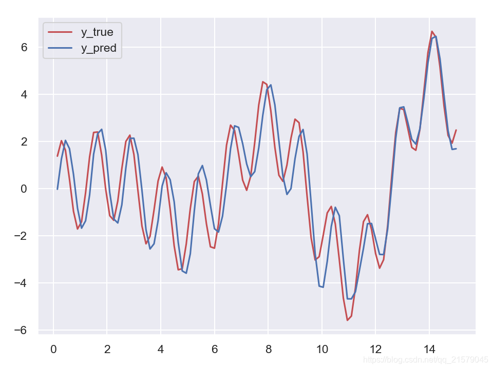
训练预测时间序列

#!/usr/bin/env python
# -*- coding: UTF-8 -*-
# coding=utf-8 

"""
@author: Li Tian
@contact: 694317828@qq.com
@software: pycharm
@file: rnn_test2.py
@time: 2019/6/18 10:11
@desc: 训练预测时间序列
"""

import tensorflow as tf
import numpy as np
from tensorflow.contrib.layers import fully_connected
from tensorflow.contrib.rnn import BasicRNNCell
from tensorflow.contrib.rnn import OutputProjectionWrapper
import pandas as pd
import matplotlib.pyplot as plt
import seaborn as sns
sns.set()


n_steps = 100
n_inputs = 1
n_neurous = 100
n_outputs = 1

learning_rate = 0.001

n_iterations = 10000
batch_size = 50

X = tf.placeholder(tf.float32, [None, n_steps, n_inputs])
y = tf.placeholder(tf.float32, [None, n_steps, n_outputs])

# 现在在每个时间迭代，有一个大小为100的输出向量，但是实际上我们需要一个单独的输出值。
# 最简单的解决方案是将单元格包装在OutputProjectionWrapper中。
# cell = OutputProjectionWrapper(BasicRNNCell(num_units=n_neurous, activation=tf.nn.relu), output_size=n_outputs)

# 用技巧提高速度
cell = BasicRNNCell(num_units=n_neurous, activation=tf.nn.relu)
rnn_outputs, states = tf.nn.dynamic_rnn(cell, X, dtype=tf.float32)
stacked_rnn_outputs = tf.reshape(rnn_outputs, [-1, n_neurous])
stacked_outputs = fully_connected(stacked_rnn_outputs, n_outputs, activation_fn=None)
outputs = tf.reshape(stacked_outputs, [-1, n_steps, n_outputs])

loss = tf.reduce_mean(tf.square(outputs - y))
optimizer = tf.train.AdamOptimizer(learning_rate=learning_rate)
training_op = optimizer.minimize(loss)

init = tf.global_variables_initializer()

X_data = np.linspace(0, 15, 101)
with tf.Session() as sess:
    init.run()
    for iteration in range(n_iterations):
        X_batch = X_data[:-1][np.newaxis, :, np.newaxis]
        y_batch = X_batch * np.sin(X_batch) / 3 + 2 * np.sin(5 * X_batch)
        sess.run(training_op, feed_dict={X: X_batch, y: y_batch})
        if iteration % 100 == 0:
            mse = loss.eval(feed_dict={X: X_batch, y: y_batch})
            print(iteration, "	MSE", mse)

    X_new = X_data[1:][np.newaxis, :, np.newaxis]
    y_true = X_new * np.sin(X_new) / 3 + 2 * np.sin(5 * X_new)
    y_pred = sess.run(outputs, feed_dict={X: X_new})

print(X_new.flatten())
print('真实结果：', y_true.flatten())
print('预测结果：', y_pred.flatten())

fig = plt.figure(dpi=150)
plt.plot(X_new.flatten(), y_true.flatten(), 'r', label='y_true')
plt.plot(X_new.flatten(), y_pred.flatten(), 'b', label='y_pred')
plt.legend()
plt.show()

运行结果

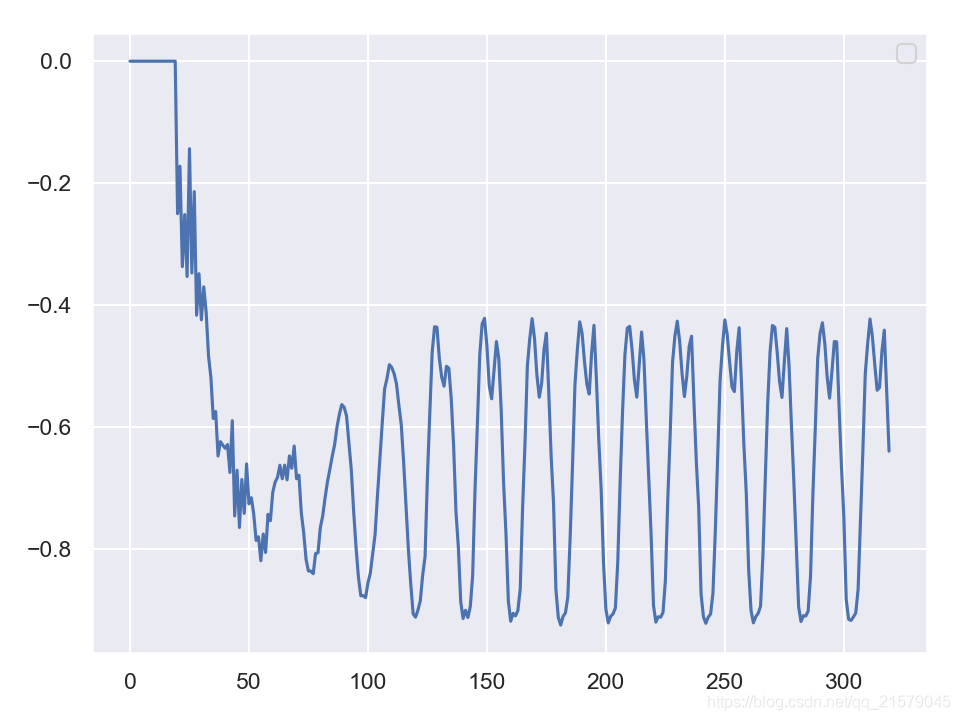
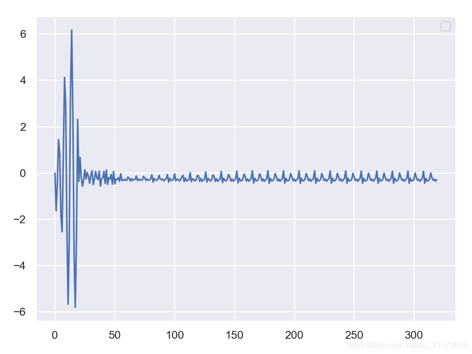
创造性的RNN

#!/usr/bin/env python
# -*- coding: UTF-8 -*-
# coding=utf-8 

"""
@author: Li Tian
@contact: 694317828@qq.com
@software: pycharm
@file: rnn_test3.py
@time: 2019/6/19 8:47
@desc: 创造性RNN
"""

import tensorflow as tf
import numpy as np
from tensorflow.contrib.layers import fully_connected
from tensorflow.contrib.rnn import BasicRNNCell
from tensorflow.contrib.rnn import OutputProjectionWrapper
import pandas as pd
import matplotlib.pyplot as plt
import seaborn as sns
sns.set()


n_steps = 20
n_inputs = 1
n_neurous = 100
n_outputs = 1

learning_rate = 0.001

n_iterations = 10000
batch_size = 50

X = tf.placeholder(tf.float32, [None, n_steps, n_inputs])
y = tf.placeholder(tf.float32, [None, n_steps, n_outputs])

# 现在在每个时间迭代，有一个大小为100的输出向量，但是实际上我们需要一个单独的输出值。
# 最简单的解决方案是将单元格包装在OutputProjectionWrapper中。
# cell = OutputProjectionWrapper(BasicRNNCell(num_units=n_neurous, activation=tf.nn.relu), output_size=n_outputs)

# 用技巧提高速度
cell = BasicRNNCell(num_units=n_neurous, activation=tf.nn.relu)
rnn_outputs, states = tf.nn.dynamic_rnn(cell, X, dtype=tf.float32)
stacked_rnn_outputs = tf.reshape(rnn_outputs, [-1, n_neurous])
stacked_outputs = fully_connected(stacked_rnn_outputs, n_outputs, activation_fn=None)
outputs = tf.reshape(stacked_outputs, [-1, n_steps, n_outputs])

loss = tf.reduce_mean(tf.square(outputs - y))
optimizer = tf.train.AdamOptimizer(learning_rate=learning_rate)
training_op = optimizer.minimize(loss)

init = tf.global_variables_initializer()

X_data = np.linspace(0, 19, 20)
with tf.Session() as sess:
    init.run()
    for iteration in range(n_iterations):
        X_batch = X_data[np.newaxis, :, np.newaxis]
        y_batch = X_batch * np.sin(X_batch) / 3 + 2 * np.sin(5 * X_batch)
        sess.run(training_op, feed_dict={X: X_batch, y: y_batch})
        if iteration % 100 == 0:
            mse = loss.eval(feed_dict={X: X_batch, y: y_batch})
            print(iteration, "	MSE", mse)

    # sequence = [0.] * n_steps
    sequence = list(y_batch.flatten())
    for iteration in range(300):
        XX_batch = np.array(sequence[-n_steps:]).reshape(1, n_steps, 1)
        y_pred = sess.run(outputs, feed_dict={X: XX_batch})
        sequence.append(y_pred[0, -1, 0])

fig = plt.figure(dpi=150)
plt.plot(sequence)
plt.legend()
plt.show()

结果1：使用零值作为种子序列

结果2：使用实例作为种子序列

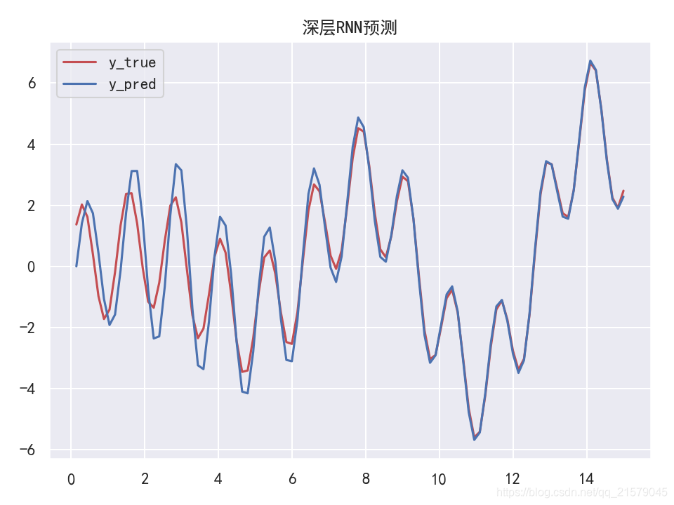
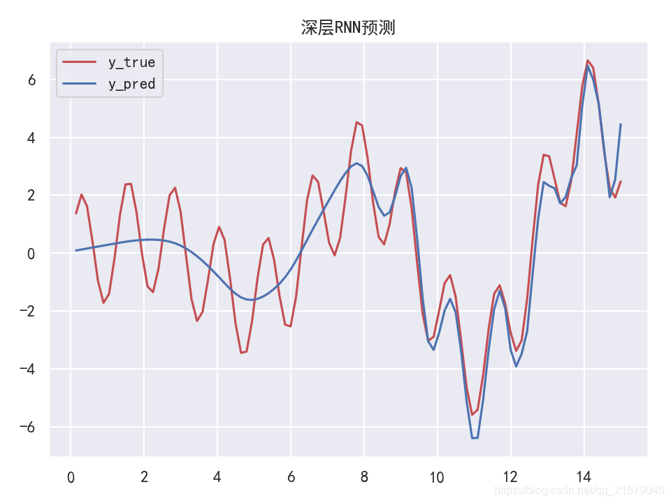
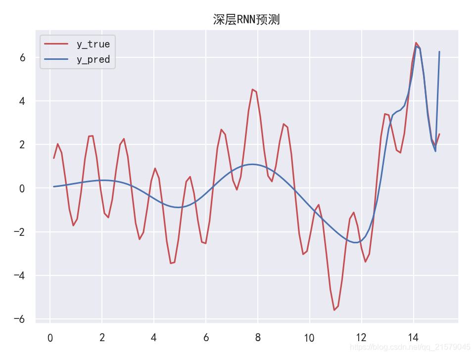
深层RNN

#!/usr/bin/env python
# -*- coding: UTF-8 -*-
# coding=utf-8 

"""
@author: Li Tian
@contact: 694317828@qq.com
@software: pycharm
@file: rnn_test4.py
@time: 2019/6/19 10:10
@desc: 深层RNN
"""

import tensorflow as tf
import numpy as np
from tensorflow.contrib.layers import fully_connected
from tensorflow.contrib.rnn import BasicRNNCell
from tensorflow.contrib.rnn import MultiRNNCell
from tensorflow.contrib.rnn import OutputProjectionWrapper
import pandas as pd
import matplotlib.pyplot as plt
import seaborn as sns
sns.set()


n_steps = 100
n_inputs = 1
n_neurous = 100
n_outputs = 1

n_layers = 10

learning_rate = 0.00001

n_iterations = 10000
batch_size = 50

X = tf.placeholder(tf.float32, [None, n_steps, n_inputs])
y = tf.placeholder(tf.float32, [None, n_steps, n_outputs])

# 现在在每个时间迭代，有一个大小为100的输出向量，但是实际上我们需要一个单独的输出值。
# 最简单的解决方案是将单元格包装在OutputProjectionWrapper中。
# cell = OutputProjectionWrapper(BasicRNNCell(num_units=n_neurous, activation=tf.nn.relu), output_size=n_outputs)

# 用技巧提高速度
# cell = BasicRNNCell(num_units=n_neurous, activation=tf.nn.relu)
# multi_layer_cell = MultiRNNCell([cell] * n_layers)
layers = [BasicRNNCell(num_units=n_neurous, activation=tf.nn.relu) for _ in range(n_layers)]
multi_layer_cell = MultiRNNCell(layers)
rnn_outputs, states = tf.nn.dynamic_rnn(multi_layer_cell, X, dtype=tf.float32)
stacked_rnn_outputs = tf.reshape(rnn_outputs, [-1, n_neurous])
stacked_outputs = fully_connected(stacked_rnn_outputs, n_outputs, activation_fn=None)
outputs = tf.reshape(stacked_outputs, [-1, n_steps, n_outputs])

loss = tf.reduce_mean(tf.square(outputs - y))
optimizer = tf.train.AdamOptimizer(learning_rate=learning_rate)
training_op = optimizer.minimize(loss)

init = tf.global_variables_initializer()

X_data = np.linspace(0, 15, 101)
with tf.Session() as sess:
    init.run()
    for iteration in range(n_iterations):
        X_batch = X_data[:-1][np.newaxis, :, np.newaxis]
        y_batch = X_batch * np.sin(X_batch) / 3 + 2 * np.sin(5 * X_batch)
        sess.run(training_op, feed_dict={X: X_batch, y: y_batch})
        if iteration % 100 == 0:
            mse = loss.eval(feed_dict={X: X_batch, y: y_batch})
            print(iteration, "	MSE", mse)

    X_new = X_data[1:][np.newaxis, :, np.newaxis]
    y_true = X_new * np.sin(X_new) / 3 + 2 * np.sin(5 * X_new)
    y_pred = sess.run(outputs, feed_dict={X: X_new})

print(X_new.flatten())
print('真实结果：', y_true.flatten())
print('预测结果：', y_pred.flatten())

plt.rcParams['font.sans-serif']=['SimHei']  # 用来正常显示中文标签
plt.rcParams['axes.unicode_minus'] = False  # 用来正常显示负号
fig = plt.figure(dpi=150)
plt.plot(X_new.flatten(), y_true.flatten(), 'r', label='y_true')
plt.plot(X_new.flatten(), y_pred.flatten(), 'b', label='y_pred')
plt.title('深层RNN预测')
plt.legend()
plt.show()

运行结果

在多个GPU中分配一个深层RNN

并没有多个GPU，所以只是整理了一下代码。。。

#!/usr/bin/env python
# -*- coding: UTF-8 -*-
# coding=utf-8 

"""
@author: Li Tian
@contact: 694317828@qq.com
@software: pycharm
@file: rnn_gpu.py
@time: 2019/6/19 12:11
@desc: 在多个GPU中分配一个深层RNN
"""

import tensorflow as tf
import numpy as np
from tensorflow.contrib.rnn import RNNCell
from tensorflow.contrib.rnn import BasicRNNCell
from tensorflow.contrib.rnn import MultiRNNCell
from tensorflow.contrib.layers import fully_connected

import matplotlib.pyplot as plt
import seaborn as sns
sns.set()


class DeviceCellWrapper(RNNCell):
    def __init__(self, device, cell):
        self._cell = cell
        self._device = device

    @property
    def state_size(self):
        return self._cell.state_size

    @property
    def output(self):
        return self._cell.output_size

    def __call__(self, inputs, state, scope=None):
        with tf.device(self._device):
            return self._cell(inputs, state, scope)


n_steps = 100
n_inputs = 1
n_neurous = 100
n_outputs = 1

n_layers = 10

learning_rate = 0.00001

n_iterations = 10000
batch_size = 50

X = tf.placeholder(tf.float32, [None, n_steps, n_inputs])
y = tf.placeholder(tf.float32, [None, n_steps, n_outputs])


devices = ['/gpu:0', '/gpu:1', '/gpu:2']
cells = [DeviceCellWrapper(dev, BasicRNNCell(num_units=n_neurous)) for dev in devices]
multi_layer_cell = MultiRNNCell(cells)
rnn_outputs,  states = tf.nn.dynamic_rnn(multi_layer_cell, X, dtype=tf.float32)

stacked_rnn_outputs = tf.reshape(rnn_outputs, [-1, n_neurous])
stacked_outputs = fully_connected(stacked_rnn_outputs, n_outputs, activation_fn=None)
outputs = tf.reshape(stacked_outputs, [-1, n_steps, n_outputs])

loss = tf.reduce_mean(tf.square(outputs - y))
optimizer = tf.train.AdamOptimizer(learning_rate=learning_rate)
training_op = optimizer.minimize(loss)

init = tf.global_variables_initializer()

X_data = np.linspace(0, 15, 101)
with tf.Session() as sess:
    init.run()
    for iteration in range(n_iterations):
        X_batch = X_data[:-1][np.newaxis, :, np.newaxis]
        y_batch = X_batch * np.sin(X_batch) / 3 + 2 * np.sin(5 * X_batch)
        sess.run(training_op, feed_dict={X: X_batch, y: y_batch})
        if iteration % 100 == 0:
            mse = loss.eval(feed_dict={X: X_batch, y: y_batch})
            print(iteration, "	MSE", mse)

    X_new = X_data[1:][np.newaxis, :, np.newaxis]
    y_true = X_new * np.sin(X_new) / 3 + 2 * np.sin(5 * X_new)
    y_pred = sess.run(outputs, feed_dict={X: X_new})

print(X_new.flatten())
print('真实结果：', y_true.flatten())
print('预测结果：', y_pred.flatten())

plt.rcParams['font.sans-serif']=['SimHei']  # 用来正常显示中文标签
plt.rcParams['axes.unicode_minus'] = False  # 用来正常显示负号
fig = plt.figure(dpi=150)
plt.plot(X_new.flatten(), y_true.flatten(), 'r', label='y_true')
plt.plot(X_new.flatten(), y_pred.flatten(), 'b', label='y_pred')
plt.title('深层RNN预测')
plt.legend()
plt.show()

应用丢弃机制

#!/usr/bin/env python
# -*- coding: UTF-8 -*-
# coding=utf-8 

"""
@author: Li Tian
@contact: 694317828@qq.com
@software: pycharm
@file: rnn_test5.py
@time: 2019/6/19 13:44
@desc: 应用丢弃机制
"""


import tensorflow as tf
import sys
import numpy as np
from tensorflow.contrib.layers import fully_connected
from tensorflow.contrib.rnn import BasicRNNCell
from tensorflow.contrib.rnn import MultiRNNCell
from tensorflow.contrib.rnn import OutputProjectionWrapper
from tensorflow.contrib.rnn import DropoutWrapper
import matplotlib.pyplot as plt
import seaborn as sns
sns.set()


is_training = (sys.argv[-1] == "train")
keep_prob = 0.5
n_steps = 100
n_inputs = 1
n_neurous = 100
n_outputs = 1

n_layers = 10

learning_rate = 0.00001

n_iterations = 10000
batch_size = 50


def make_rnn_cell():
    return BasicRNNCell(num_units=n_neurous, activation=tf.nn.relu)


def make_drop_cell():
    return DropoutWrapper(make_rnn_cell(), input_keep_prob=keep_prob)


X = tf.placeholder(tf.float32, [None, n_steps, n_inputs])
y = tf.placeholder(tf.float32, [None, n_steps, n_outputs])

# 现在在每个时间迭代，有一个大小为100的输出向量，但是实际上我们需要一个单独的输出值。
# 最简单的解决方案是将单元格包装在OutputProjectionWrapper中。
# cell = OutputProjectionWrapper(BasicRNNCell(num_units=n_neurous, activation=tf.nn.relu), output_size=n_outputs)

# 用技巧提高速度
layers = [make_rnn_cell() for _ in range(n_layers)]
if is_training:
    layers = [make_drop_cell() for _ in range(n_layers)]

multi_layer_cell = MultiRNNCell(layers)
rnn_outputs, states = tf.nn.dynamic_rnn(multi_layer_cell, X, dtype=tf.float32)
stacked_rnn_outputs = tf.reshape(rnn_outputs, [-1, n_neurous])
stacked_outputs = fully_connected(stacked_rnn_outputs, n_outputs, activation_fn=None)
outputs = tf.reshape(stacked_outputs, [-1, n_steps, n_outputs])

loss = tf.reduce_mean(tf.square(outputs - y))
optimizer = tf.train.AdamOptimizer(learning_rate=learning_rate)
training_op = optimizer.minimize(loss)

init = tf.global_variables_initializer()

X_data = np.linspace(0, 15, 101)

'''
# 应用丢弃机制
saver = tf.train.Saver()

with tf.Session() as sess:
    if is_training:
        init.run()
        for iteration in range(n_iterations):
            # train the model
        save_path = saver.save(sess, "./my_model.ckpt")
    else:
        saver.restore(sess, "./my_model.ckpt")
        # use the model
'''

with tf.Session() as sess:
    init.run()
    for iteration in range(n_iterations):
        X_batch = X_data[:-1][np.newaxis, :, np.newaxis]
        y_batch = X_batch * np.sin(X_batch) / 3 + 2 * np.sin(5 * X_batch)
        sess.run(training_op, feed_dict={X: X_batch, y: y_batch})
        if iteration % 100 == 0:
            mse = loss.eval(feed_dict={X: X_batch, y: y_batch})
            print(iteration, "	MSE", mse)

    X_new = X_data[1:][np.newaxis, :, np.newaxis]
    y_true = X_new * np.sin(X_new) / 3 + 2 * np.sin(5 * X_new)
    y_pred = sess.run(outputs, feed_dict={X: X_new})

print(X_new.flatten())
print('真实结果：', y_true.flatten())
print('预测结果：', y_pred.flatten())

plt.rcParams['font.sans-serif']=['SimHei']  # 用来正常显示中文标签
plt.rcParams['axes.unicode_minus'] = False  # 用来正常显示负号
fig = plt.figure(dpi=150)
plt.plot(X_new.flatten(), y_true.flatten(), 'r', label='y_true')
plt.plot(X_new.flatten(), y_pred.flatten(), 'b', label='y_pred')
plt.title('深层RNN预测')
plt.legend()
plt.show()

运行结果

LSTM单元

四个不同的全连接层：主层：tanh，直接输出$y_t和h_t$；忘记门限：logitstic，控制着哪些长期状态应该被丢弃；输入门限：控制着主层的哪些部分会被加入到长期状态（这就是“部分存储”的原因）；输出门限：控制着哪些长期状态应该在这个时间迭代被读取和输出（$h_t和y_t$）。

#!/usr/bin/env python
# -*- coding: UTF-8 -*-
# coding=utf-8 

"""
@author: Li Tian
@contact: 694317828@qq.com
@software: pycharm
@file: lstm_test1.py
@time: 2019/6/19 14:51
@desc: LSTM单元
"""

import tensorflow as tf
import sys
import numpy as np
from tensorflow.contrib.layers import fully_connected
from tensorflow.contrib.rnn import BasicLSTMCell
from tensorflow.contrib.rnn import MultiRNNCell
from tensorflow.contrib.rnn import OutputProjectionWrapper
from tensorflow.contrib.rnn import DropoutWrapper
import matplotlib.pyplot as plt
import seaborn as sns
sns.set()


is_training = (sys.argv[-1] == "train")
keep_prob = 0.5
n_steps = 100
n_inputs = 1
n_neurous = 100
n_outputs = 1

n_layers = 5

learning_rate = 0.00001

n_iterations = 10000
batch_size = 50


def make_rnn_cell():
    return BasicLSTMCell(num_units=n_neurous, activation=tf.nn.relu)


def make_drop_cell():
    return DropoutWrapper(make_rnn_cell(), input_keep_prob=keep_prob)


X = tf.placeholder(tf.float32, [None, n_steps, n_inputs])
y = tf.placeholder(tf.float32, [None, n_steps, n_outputs])

# 现在在每个时间迭代，有一个大小为100的输出向量，但是实际上我们需要一个单独的输出值。
# 最简单的解决方案是将单元格包装在OutputProjectionWrapper中。
# cell = OutputProjectionWrapper(BasicRNNCell(num_units=n_neurous, activation=tf.nn.relu), output_size=n_outputs)

# 用技巧提高速度
layers = [make_rnn_cell() for _ in range(n_layers)]
# if is_training:
#     layers = [make_drop_cell() for _ in range(n_layers)]

multi_layer_cell = MultiRNNCell(layers)
rnn_outputs, states = tf.nn.dynamic_rnn(multi_layer_cell, X, dtype=tf.float32)
stacked_rnn_outputs = tf.reshape(rnn_outputs, [-1, n_neurous])
stacked_outputs = fully_connected(stacked_rnn_outputs, n_outputs, activation_fn=None)
outputs = tf.reshape(stacked_outputs, [-1, n_steps, n_outputs])

loss = tf.reduce_mean(tf.square(outputs - y))
optimizer = tf.train.AdamOptimizer(learning_rate=learning_rate)
training_op = optimizer.minimize(loss)

init = tf.global_variables_initializer()

X_data = np.linspace(0, 15, 101)

with tf.Session() as sess:
    init.run()
    for iteration in range(n_iterations):
        X_batch = X_data[:-1][np.newaxis, :, np.newaxis]
        y_batch = X_batch * np.sin(X_batch) / 3 + 2 * np.sin(5 * X_batch)
        sess.run(training_op, feed_dict={X: X_batch, y: y_batch})
        if iteration % 100 == 0:
            mse = loss.eval(feed_dict={X: X_batch, y: y_batch})
            print(iteration, "	MSE", mse)

    X_new = X_data[1:][np.newaxis, :, np.newaxis]
    y_true = X_new * np.sin(X_new) / 3 + 2 * np.sin(5 * X_new)
    y_pred = sess.run(outputs, feed_dict={X: X_new})

print(X_new.flatten())
print('真实结果：', y_true.flatten())
print('预测结果：', y_pred.flatten())

plt.rcParams['font.sans-serif']=['SimHei']  # 用来正常显示中文标签
plt.rcParams['axes.unicode_minus'] = False  # 用来正常显示负号
fig = plt.figure(dpi=150)
plt.plot(X_new.flatten(), y_true.flatten(), 'r', label='y_true')
plt.plot(X_new.flatten(), y_pred.flatten(), 'b', label='y_pred')
plt.title('深层RNN预测')
plt.legend()
plt.show()

运行结果

窥视孔连接

窥视孔连接（peephole connections）：LSTM变体，当前一个长期状态$c_{(t-1)}$作为输入传入忘记门限和输入门限，当前的长期状态$c_{(t)}$作为输入传出门限控制器。

#!/usr/bin/env python
# -*- coding: UTF-8 -*-
# coding=utf-8 

"""
@author: Li Tian
@contact: 694317828@qq.com
@software: pycharm
@file: lstm_test2.py
@time: 2019/6/19 16:36
@desc: 窥视孔连接
"""

import tensorflow as tf
import numpy as np
from tensorflow.contrib.layers import fully_connected
from tensorflow.contrib.rnn import LSTMCell
from tensorflow.contrib.rnn import MultiRNNCell
from tensorflow.contrib.rnn import OutputProjectionWrapper
import pandas as pd
import matplotlib.pyplot as plt
import seaborn as sns
sns.set()


n_steps = 100
n_inputs = 1
n_neurous = 100
n_outputs = 1

n_layers = 10

learning_rate = 0.00001

n_iterations = 10000
batch_size = 50

X = tf.placeholder(tf.float32, [None, n_steps, n_inputs])
y = tf.placeholder(tf.float32, [None, n_steps, n_outputs])

# 现在在每个时间迭代，有一个大小为100的输出向量，但是实际上我们需要一个单独的输出值。
# 最简单的解决方案是将单元格包装在OutputProjectionWrapper中。
# cell = OutputProjectionWrapper(BasicRNNCell(num_units=n_neurous, activation=tf.nn.relu), output_size=n_outputs)

# 用技巧提高速度
# cell = BasicRNNCell(num_units=n_neurous, activation=tf.nn.relu)
# multi_layer_cell = MultiRNNCell([cell] * n_layers)
layers = [LSTMCell(num_units=n_neurous, activation=tf.nn.relu, use_peepholes=True) for _ in range(n_layers)]
multi_layer_cell = MultiRNNCell(layers)
rnn_outputs, states = tf.nn.dynamic_rnn(multi_layer_cell, X, dtype=tf.float32)
stacked_rnn_outputs = tf.reshape(rnn_outputs, [-1, n_neurous])
stacked_outputs = fully_connected(stacked_rnn_outputs, n_outputs, activation_fn=None)
outputs = tf.reshape(stacked_outputs, [-1, n_steps, n_outputs])

loss = tf.reduce_mean(tf.square(outputs - y))
optimizer = tf.train.AdamOptimizer(learning_rate=learning_rate)
training_op = optimizer.minimize(loss)

init = tf.global_variables_initializer()

X_data = np.linspace(0, 15, 101)
with tf.Session() as sess:
    init.run()
    for iteration in range(n_iterations):
        X_batch = X_data[:-1][np.newaxis, :, np.newaxis]
        y_batch = X_batch * np.sin(X_batch) / 3 + 2 * np.sin(5 * X_batch)
        sess.run(training_op, feed_dict={X: X_batch, y: y_batch})
        if iteration % 100 == 0:
            mse = loss.eval(feed_dict={X: X_batch, y: y_batch})
            print(iteration, "	MSE", mse)

    X_new = X_data[1:][np.newaxis, :, np.newaxis]
    y_true = X_new * np.sin(X_new) / 3 + 2 * np.sin(5 * X_new)
    y_pred = sess.run(outputs, feed_dict={X: X_new})

print(X_new.flatten())
print('真实结果：', y_true.flatten())
print('预测结果：', y_pred.flatten())

plt.rcParams['font.sans-serif']=['SimHei']  # 用来正常显示中文标签
plt.rcParams['axes.unicode_minus'] = False  # 用来正常显示负号
fig = plt.figure(dpi=150)
plt.plot(X_new.flatten(), y_true.flatten(), 'r', label='y_true')
plt.plot(X_new.flatten(), y_pred.flatten(), 'b', label='y_pred')
plt.title('深层RNN预测')
plt.legend()
plt.show()

运行结果

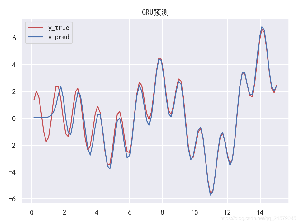
GRU单元

GRU单元是LSTM的简化版本，其主要简化了：

两个状态向量合并为一个向量$h_{(t)}$。
一个门限控制器同时控制忘记门限和输入门限。如果门限控制器的输出是1，那么输入门限打开而忘记门限关闭。如果输出是0，则刚好相反。换句话说，无论何时需要存储一个记忆，它将被存在的位置将首先被擦除。这实际上是LSTM单元的一个常见变体。
没有输出门限。在每个时间迭代，输出向量的全部状态被直接输出。然而，GRU有一个新的门限控制器来控制前一个状态的哪部分将显示给主层。

GRU 是新一代的循环神经网络，与 LSTM 非常相似。与 LSTM 相比，GRU 去除掉了细胞状态，使用隐藏状态来进行信息的传递。它只包含两个门：更新门和重置门。
更新门：更新门的作用类似于 LSTM 中的遗忘门和输入门。它决定了要忘记哪些信息以及哪些新信息需要被添加。
重置门：重置门用于决定遗忘先前信息的程度。
GRU 的张量运算较少，因此它比 LSTM 的训练更快一下。很难去判定这两者到底谁更好，研究人员通常会两者都试一下，然后选择最合适的。

#!/usr/bin/env python
# -*- coding: UTF-8 -*-
# coding=utf-8 

"""
@author: Li Tian
@contact: 694317828@qq.com
@software: pycharm
@file: gru_test1.py
@time: 2019/6/19 17:07
@desc: GRU单元
"""

import tensorflow as tf
import numpy as np
from tensorflow.contrib.layers import fully_connected
from tensorflow.contrib.rnn import GRUCell
from tensorflow.contrib.rnn import MultiRNNCell
from tensorflow.contrib.rnn import OutputProjectionWrapper
import pandas as pd
import matplotlib.pyplot as plt
import seaborn as sns
sns.set()


n_steps = 100
n_inputs = 1
n_neurous = 100
n_outputs = 1

n_layers = 10

learning_rate = 0.00001

n_iterations = 10000
batch_size = 50

X = tf.placeholder(tf.float32, [None, n_steps, n_inputs])
y = tf.placeholder(tf.float32, [None, n_steps, n_outputs])

# 现在在每个时间迭代，有一个大小为100的输出向量，但是实际上我们需要一个单独的输出值。
# 最简单的解决方案是将单元格包装在OutputProjectionWrapper中。
# cell = OutputProjectionWrapper(BasicRNNCell(num_units=n_neurous, activation=tf.nn.relu), output_size=n_outputs)

# 用技巧提高速度
# cell = BasicRNNCell(num_units=n_neurous, activation=tf.nn.relu)
# multi_layer_cell = MultiRNNCell([cell] * n_layers)
layers = [GRUCell(num_units=n_neurous, activation=tf.nn.relu) for _ in range(n_layers)]
multi_layer_cell = MultiRNNCell(layers)
rnn_outputs, states = tf.nn.dynamic_rnn(multi_layer_cell, X, dtype=tf.float32)
stacked_rnn_outputs = tf.reshape(rnn_outputs, [-1, n_neurous])
stacked_outputs = fully_connected(stacked_rnn_outputs, n_outputs, activation_fn=None)
outputs = tf.reshape(stacked_outputs, [-1, n_steps, n_outputs])

loss = tf.reduce_mean(tf.square(outputs - y))
optimizer = tf.train.AdamOptimizer(learning_rate=learning_rate)
training_op = optimizer.minimize(loss)

init = tf.global_variables_initializer()

X_data = np.linspace(0, 15, 101)
with tf.Session() as sess:
    init.run()
    for iteration in range(n_iterations):
        X_batch = X_data[:-1][np.newaxis, :, np.newaxis]
        y_batch = X_batch * np.sin(X_batch) / 3 + 2 * np.sin(5 * X_batch)
        sess.run(training_op, feed_dict={X: X_batch, y: y_batch})
        if iteration % 100 == 0:
            mse = loss.eval(feed_dict={X: X_batch, y: y_batch})
            print(iteration, "	MSE", mse)

    X_new = X_data[1:][np.newaxis, :, np.newaxis]
    y_true = X_new * np.sin(X_new) / 3 + 2 * np.sin(5 * X_new)
    y_pred = sess.run(outputs, feed_dict={X: X_new})

print(X_new.flatten())
print('真实结果：', y_true.flatten())
print('预测结果：', y_pred.flatten())

plt.rcParams['font.sans-serif']=['SimHei']  # 用来正常显示中文标签
plt.rcParams['axes.unicode_minus'] = False  # 用来正常显示负号
fig = plt.figure(dpi=150)
plt.plot(X_new.flatten(), y_true.flatten(), 'r', label='y_true')
plt.plot(X_new.flatten(), y_pred.flatten(), 'b', label='y_pred')
plt.title('GRU预测')
plt.legend()
plt.show()

运行结果

参考链接：深入理解LSTM，窥视孔连接，GRU

更好的参考链接：GRU与LSTM总结

其他变形的LSTM网络总结

参考链接：直观理解LSTM（长短时记忆网络）

窥视孔连接LSTM

一种流行的LSTM变种，由Gers和Schmidhuber （2000）提出，加入了“窥视孔连接”（peephole connections）。这意味着门限层也将单元状态作为输入。
耦合遗忘输入门限的LSTM

就是使用耦合遗忘和输入门限。我们不单独决定遗忘哪些、添加哪些新信息，而是一起做出决定。在输入的时候才进行遗忘。在遗忘某些旧信息时才将新值添加到状态中。
门限递归单元（GRU）

它将遗忘和输入门限结合输入到单个“更新门限”中。同样还将单元状态和隐藏状态合并，并做出一些其他变化。所得模型比标准LSTM模型要简单，这种做法越来越流行。

部分课后题的摘抄

在构建RNN时使用dynamic_rnn()而不是static_rnn()的优势是什么？
1. 它基于while_loop()操作，可以在反向传播期间将GPU内存交互到CPU内存，从而避免了内存溢出。
2. 它更加易于使用，因为其采取单张量作为输入和输出（覆盖所有时间步长），而不是一个张量列表（每个时间一个步长）。不需要入栈、出栈，或转置。
3. 它产生的图形更小，更容易在TensorBoard中可视化。
如何处理变长输入序列？变长输出序列又会怎么样？
1. 为了处理可变长度的输入序列，最简单的方法是在调用static_rnn()或dynamic_rnn()方法时传入sequence_length参数。另一个方法是填充长度较小的输入（比如，用0填充）来使其与最大输入长度相同（这可能比第一种方法快，因为所有输入序列具有相同的长度）。
2. 为了处理可变长度的输出序列，如果事先知道每个输出序列的长度，就可以使用sequence_length参数（例如，序列到序列RNN使用暴力评分标记视频中的每一帧：输出序列和输入序列长度完全一致）。如果事先不知道输出序列的长度，则可以使用填充方法：始终输出相同大小的序列，但是忽略end-of-sequence标记之后的任何输出（在计算成本函数时忽略它们）。
在多个GPU之间分配训练和执行层次RNN的常见方式是什么？

为了在多个GPU直接分配训练并执行深度RNN，一个常用的简单技术是将每个层放在不同的GPU上。

我的CSDN：https://blog.csdn.net/qq_21579045

我的博客园：https://www.cnblogs.com/lyjun/

我的Github：https://github.com/TinyHandsome

纸上得来终觉浅，绝知此事要躬行~

欢迎大家过来OB~

by 李英俊小朋友

查看全文

相关阅读:
哈希表
 矩阵加速（数列）
线段树
 python
vue 中防抖
 Windows版本与Internet Explorer版本对照
 一个怂女婿的成长笔记【二十三】
一个怂女婿的成长笔记【二十一】
vue xml数据格式化展示，展示在textarea里可编辑，和高亮处理方法
 substring 截取第三个字符（/）后的字符串

原文地址：https://www.cnblogs.com/lyjun/p/11057371.html

第14章 循环神经网络

第14章 循环神经网络

写在前面

TensorFlow中的基本RNN

通过时间静态展开

通过时间动态展开

处理长度可变输入序列

处理长度可变输出序列

训练RNN

训练序列分类器

训练预测时间序列

创造性的RNN

深层RNN

在多个GPU中分配一个深层RNN

应用丢弃机制

LSTM单元

窥视孔连接

GRU单元

其他变形的LSTM网络总结

部分课后题的摘抄

第14章循环神经网络

第14章循环神经网络