[Reinforcement Learning] Model-Free Control

上篇总结了 Model-Free Predict 问题及方法，本文内容介绍 Model-Free Control 方法，即 "Optimise the value function of an unknown MDP"。

在这里说明下，Model-Free Predict/Control 不仅适用于 Model-Free 的情况，其同样适用于 MDP 已知的问题：

• MDP model is unknown, but experience can be sampled.
• MDP model is known, but is too big to use, except by samples.

在正式介绍 Model-Free Control 方法之前，我们先介绍下 On-policy Learning 及 Off-policy Learning。

On-policy Learning vs. Off-policy Learning

On-policy Learning：

• "Learn on the job"
• Learn about policy (pi) from experience sampled from (pi)（即采样的策略与学习的策略一致）

Off-policy Learning：

• "Look over someone's shoulder"
• Learn about policy (pi) from experience sampled from (mu)（即采样的策略与学习的策略不一致）

On-Policy Monte-Carlo Learning

Generalized Policy Iteration

具体的 Control 方法，在《动态规划》一文中我们提到了 Model-based 下的广义策略迭代 GPI 框架，那在 Model-Free 情况下是否同样适用呢？
如下图为 Model-based 下的广义策略迭代 GPI 框架，主要分两部分：策略评估及基于 Greedy 策略的策略提升。


Model-Free 策略评估

在《Model-Free Predict》中我们分别介绍了两种 Model-Free 的策略评估方法：MC 和 TD。我们先讨论使用 MC 情况下的 Model-Free 策略评估。
如上图GPI框架所示：

• 基于 (V(s)) 的贪婪策略提升需要 MDP 已知：

[pi'(s) = argmax_{ain A}Bigl(R_{s}^{a}+P_{ss'}^{a}V(s')Bigr) ]

• 基于 (Q(s, a)) 的贪婪策略提升不需要 MDP 已知，即 Model-Free：

[pi'(s) = argmax_{ain A}Q(s, a) ]

因此 Model-Free 下需要对 (Q(s, a)) 策略评估，整个GPI策略迭代也要基于 (Q(s, a))。

Model-Free 策略提升

确定了策略评估的对象，那接下来要考虑的就是如何基于策略评估的结果 (Q(s, a)) 进行策略提升。
由于 Model-Free 的策略评估基于对经验的 samples（即评估的 (q(s, a)) 存在 bias），因此我们在这里不采用纯粹的 greedy 策略，防止因为策略评估的偏差导致整个策略迭代进入局部最优，而是采用具有 explore 功能的 (epsilon)-greedy 算法：

[pi(a|s) = egin{cases} &frac{epsilon}{m} + 1 - epsilon, & ext{if } a^*=argmax_{ain A}Q(s, a)\ &frac{epsilon}{m}, & ext{otherwise} end{cases} ]

因此，我们确定了 Model-Free 下的 Monto-Carlo Control：


GLIE

先直接贴下David的课件，GLIE 介绍如下：


对于 (epsilon)-greedy 算法而言，如果 (epsilon) 随着迭代次数逐步减为0，那么 (epsilon)-greedy 是 GLIE，即：

[epsilon_{k} = frac{1}{k} ]

GLIE Monto-Carlo Control

GLIE Monto-Carlo Control：

• 对于 episode 中的每个状态 (S_{t}) 和动作 (A_t)：

[N(S_t, A_t) ← N(S_t, A_t) + 1 \ Q(S_t, A_t) ← Q(S_t, A_t) + frac{1}{N(S_t, A_t)}(G_t - Q(S_t, A_t)) ]

• 基于新的动作价值函数提升策略：

[epsilon ← frac{1}{k}\ pi ← epsilon ext{-greedy}(Q) ]

定理：GLIE Monto-Carlo Control 收敛到最优的动作价值函数，即：(Q(s, a) → q_*(s, a))。

On-Policy Temporal-Difference Learning

Sarsa

我们之前总结过 TD 相对 MC 的优势：

• 低方差
• Online
• 非完整序列

那么一个很自然的想法就是在整个控制闭环中用 TD 代替 MC：

• 使用 TD 来计算 (Q(S, A))
• 仍然使用 (epsilon)-greedy 策略提升
• 每一个 step 进行更新

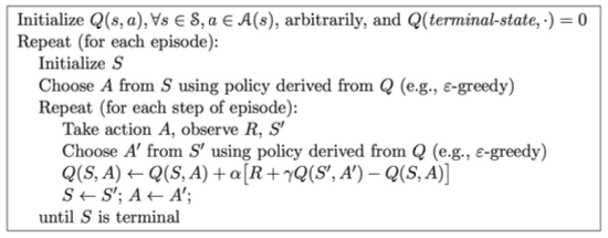
通过上述改变就使得 On-Policy 的蒙特卡洛方法变成了著名的 Sarsa。

• 更新动作价值函数


- Control


Sarsa算法的伪代码如下：

Sarsa(λ)

n-step Sarsa returns 可以表示如下：
(n=1) 时：(q_{t}^{(1)} = R_{t+1} + gamma Q(S_{t+1}))
(n=2) 时：(q_{t}^{(2)} = R_{t+1} + gamma R_{t+2} + gamma^2 Q(S_{t+2}))
...
(n=infty) 时：(q_{t}^{infty} = R_{t+1} + gamma R_{t+2} + ... + gamma^{T-1} R_T)
因此，n-step return (q_{t}^{(n)} = R_{t+1} + gamma R_{t+2} + ... + gamma^{n}Q(S_{t+n}))

n-step Sarsa 更新公式：

[Q(S_t, A_t) ← Q(S_t, A_t) + alpha (q_t^{(n)} - Q(S_t, A_t)) ]

具体的 Sarsa(λ) 算法伪代码如下：

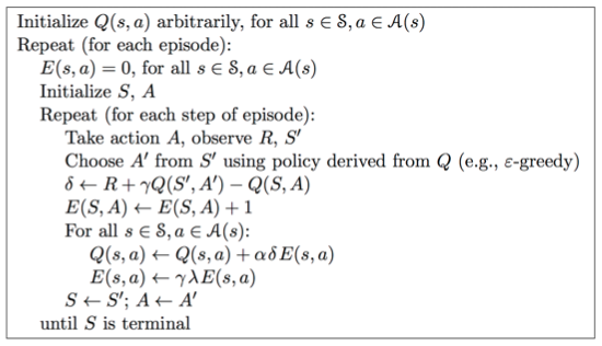
其中 (E(s, a)) 为资格迹。

下图为 Sarsa(λ) 用于 Gridworld 例子的示意图：


Off-Policy Learning

Off-Policy Learning 的特点是评估目标策略 (pi(a|s)) 来计算 (v_{pi}(s)) 或者 (q_{pi}(s, a))，但是跟随行为策略 ({S_1, A_1, R_2, ..., S_T}simmu(a|s))。

Off-Policy Learning 有什么意义？

• Learn from observing humans or other agents
• Re-use experience generated from old policies (pi_1, pi_2, ..., pi_{t-1})
• Learn about optimal policy while following exploratory policy
• Learn about multiple policies while following one policy

重要性采样

重要性采样的目的是：Estimate the expectation of a different distribution。

[egin{align} E_{Xsim P}[f(X)] &= sum P(X)f(X)\ &= sum Q(X)frac{P(X)}{Q(X)}f(X)\ &= E_{Xsim Q}[frac{P(X)}{Q(X)}f(X)] end{align} ]

Off-Policy MC 重要性采样

使用策略 (pi) 产生的 return 来评估 (mu)：

[G_t^{pi/mu} = frac{pi(A_t|S_t)}{mu(A_t|S_t)} frac{pi(A_{t+1}|S_{t+1})}{mu(A_{t+1}|S_{t+1})}...frac{pi(A_T|S_T)}{mu(A_T|S_T)}G_t ]

朝着正确的 return 方向去更新价值：

[V(S_t) ← V(S_t) + alphaBigl(color{Red}{G_t^{pi/mu}}-V(S_t)Bigr) ]

需要注意两点：

• Cannot use if (mu) is zero when (pi) is non-zero
• 重要性采样会显著性地提升方差

Off-Policy TD 重要性采样

TD 是单步的，所以使用策略 (pi) 产生的 TD targets 来评估 (mu)：

[V(S_t) ← V(S_t) + alphaBigl(frac{pi(A_t|S_t)}{mu(A_t|S_t)}(R_{t+1}+gamma V(S_{t+1}))-V(S_t)Bigr) ]

• 方差比MC版本的重要性采样低很多

Q-Learning

前面分别介绍了对价值函数 (V(s)) 进行 off-policy 学习，现在我们讨论如何对动作价值函数 (Q(s, a)) 进行 off-policy 学习：

• 不需要重要性采样
• 使用行为策略选出下一步的动作：(A_{t+1}simmu(·|S_t))
• 但是仍需要考虑另一个后继动作：(A'simpi(·|S_t))
• 朝着另一个后继动作的价值更新 (Q(S_t, A_t))：

[Q(S_t, A_t) ← Q(S_t, A_t) + alphaBigl(R_{t+1}+gamma Q(S_{t+1}, A')-Q(S_t, A_t)Bigr) ]

讨论完对动作价值函数的学习，我们接着看如何通过 Q-Learning 进行 Control：

• 行为策略和目标策略均改进
• 目标策略 (pi) 以greedy方式改进：

[pi(S_t) = argmax_{a'}Q(S_{t+1}, a') ]

• 行为策略 (mu) 以 (epsilon)-greedy 方式改进
• Q-Learning target：

[egin{align} &R_{t+1}+gamma Q(S_{t+1}, A')\ =&R_{t+1}+gamma QBigl(S_{t+1}, argmax_{a'}Q(S_{t+1}, a')Bigr)\ =&R_{t+1}+max_{a'}gamma Q(S_{t+1}, a') end{align} ]

Q-Learning 的 backup tree 如下所示：


关于 Q-Learning 的结论：

Q-learning control converges to the optimal action-value function, (Q(s, a)→q_*(s, a))

Q-Learning 算法具体的伪代码如下：


对比 Sarsa 与 Q-Learning 可以发现两个最重要的区别：

• TD target 公式不同
• Q-Learning 中下一步的动作从行为策略中选出，而不是目标策略

DP vs. TD

两者的区别见下表：

 

Reference

[1] Reinforcement Learning: An Introduction, Richard S. Sutton and Andrew G. Barto, 2018
[2] David Silver's Homepage