course link: https://class.coursera.org/fmri1-001
Part 1
❤ Three fundmental goals in fMRI:
localization (brain mapping approach: task comparison, brain-behavior correlation, information-based mapping);
connectivity (functional connectivity (seed-based), effectivity connectivity (DCM), multivariate connectivity (ICA, PCA, graph theory));
prediction (use the brain activities to predict something such as behavior)
❤ fMRI data structure:
TR: temporal resolution
Sturctural images:T1, WM<GM<CSF (longitudinal relaxation)
Functional images: T2* images
T2: teanscerse reliaxation
❤ fmri data structure
Field of view (FOV): to what extent of view in each direction we can see the brain
Slice thickness
eg. If the FOC is 192 mm, matrix size is 64 mm (the area of each slice), the slice thickness is 3 mm, then voxel size: 192mm (FOV)/64 (matrix size)*3 (slice thickness) = 3*3*3 mm voxel size (the last 3 means slice thickness)
hierarchy: Experiment-subjects-session-run-volume-slice-voxel
❤ Statistical map: the colors indicate reliable, non-zero effects
❤ Reverse inference: observed brain actives -> the feeling
One fallacy: if P->Q, Q, therefore P (true only if P is the only factor leads to Q)
❤ For regional brain activation to have high positive predictive value:
- It must respond consistently to the task/state (high sentivitivity);
- It must respond only to the task/state (high specificity).
Part 2
course link: https://class.coursera.org/fmri1-001
❤ T1 time
WM = 600;
GM = 1000;
CSF = 3000.
❤ Terms relating to time
TR: how often we excite the nuclei;
TE: how soon after exciation we begin data collection.
❤ K-space
K-space is frequency space.
Doing inverse Fourier transformation on points in k-space could reconstruct brain image we need.
Each individual point in image space depends on all points in k-space (in other words, the value of the points in k-space tells us its relative contribution in reconstruct the brain image).
"Low spatial frequencies represent parts of the object that change in a spatially slow manner (Contrast); high spatial frequencies represent small structures whose size is on the same order as the voxel size (Tissue boundaries)." -- the center points in the k-space contribute most of the brain image, while the outskirt part mostly contribute to the sketch of the brain.
Part 3
❤ BOLD signal
- Oxyhemoglobin is diamagnetic; while deoxyhemoglobin is paramagnetic (distort the magetic fields, and suppress the MR signal - when deoxyhemoglobin decrease, then the T2*-weighted signal increase).
- Bold signal often corresponds relatively closely to the local field potential (LFP - often reflect the integrated post-synaptic activiy across a group of neurons) - the electrical field potentional surrounding a group of cells.
- Bold signal does not always reflect changes in neuron activity.
❤ Basic quality control
- SNR (signal-to-noise ratio): a basic measure of effect size.
- CNR (contrast-to-noise ratio)
The two measurements can be calculated at both spatial and temporal level. Note that for temporally detrended data, the temporal SNR (or functional SNR) is also called Signal-to-Fluctuation-Noise Ratio (SFNR). Temporal CNR is also signal sentivity.
- Bold response is non-linear, which may cause nonlinear 'saturation'. This effect can be reduced by increasing the intervals between two stimuli.
❤ fMRI artefacts and non-signal-related noise
- Drift (low frequency noise)
Slow changes in voxel intersity over time - scanner instabilities and aliased physiological noise. Should be taken care about when pre-process images and conduct statistical analysis.
To aviod drift the experiment design should be fast.
-Motion
Should be taken care about when pre-process images and conduct statistical analysis. Only motion correction in pre-processing steps is not enough.
- Respiration and heart rate
TR that is too low may give rise to aliasing.
Part 6 - GLM
- Statistical analysis under certain circumstances:

- Pay attention that the first colume of design matrix should be 1, in correspondance to β0;
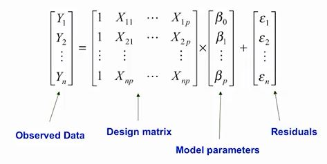
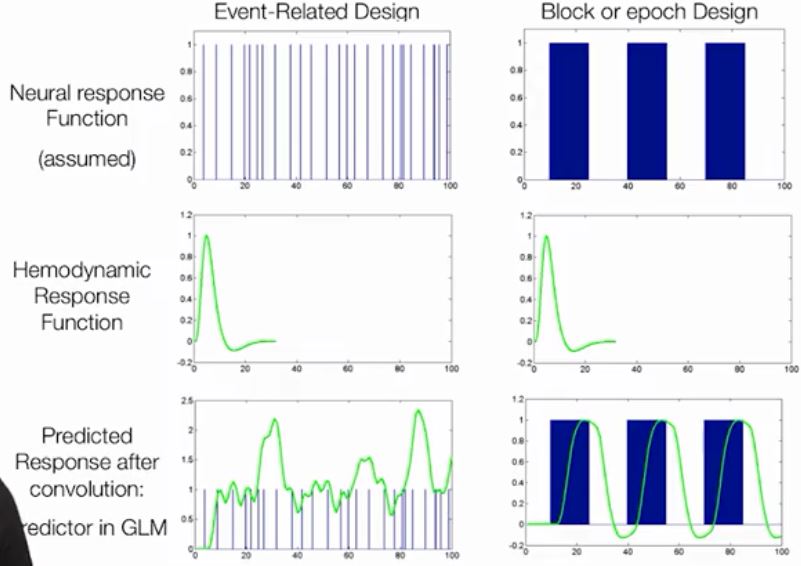
- Build a certian GLM model: assume a LTI (linear time invariant) system (because HRF is fixed and will not change with time), and the predictors (Xs) should be the neural response function convolved with HRF;
- Mass univariate analysis: assume each voxel in the brain responding independently, and build a GLM for them each for analysis;
- Contrast: vector of weights, used to perform statistical analysis (c'*β = a, a is h in statistical analysis). Usually sum(c) should equal to 0 for the convenience to conduct statistical analysis of H0 = 0.
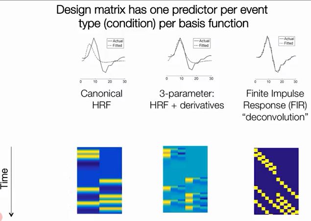
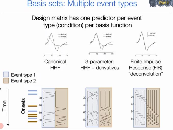
- Using one sigle shaped curve to fit the HRF has imperfictions: actually HRF varies across brain regions and experiment paradigm. Three ways to model HRF:
❤ Parameters estimation (actually we don't have to care about these the details)
- Based on the assumption below:
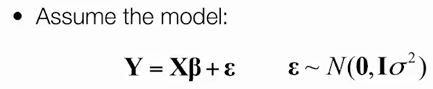
The following computation is based on two kind of hypothesis: ε is normally distributed at the mean zero and is IID (Independent and identically distributed) (then the variance-covariance matrix V can be considered as I(σ^2)) or not.
Then we have:

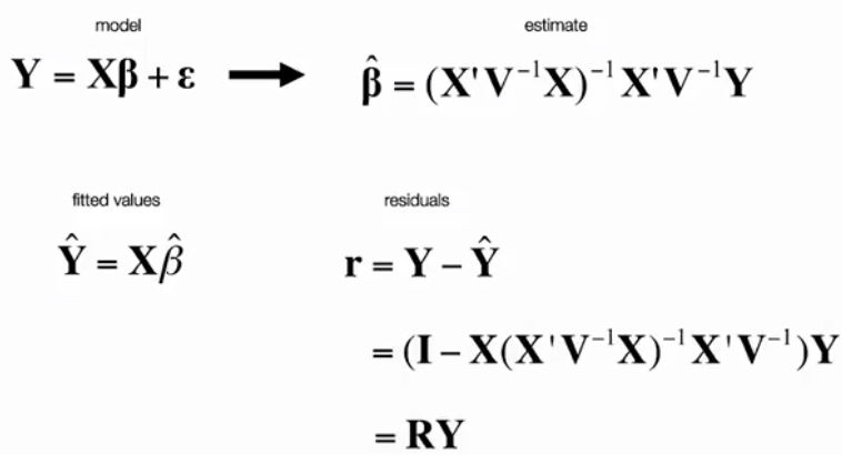

- Specific computation equations for T and F-test in SPM:
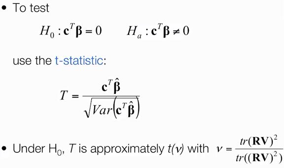

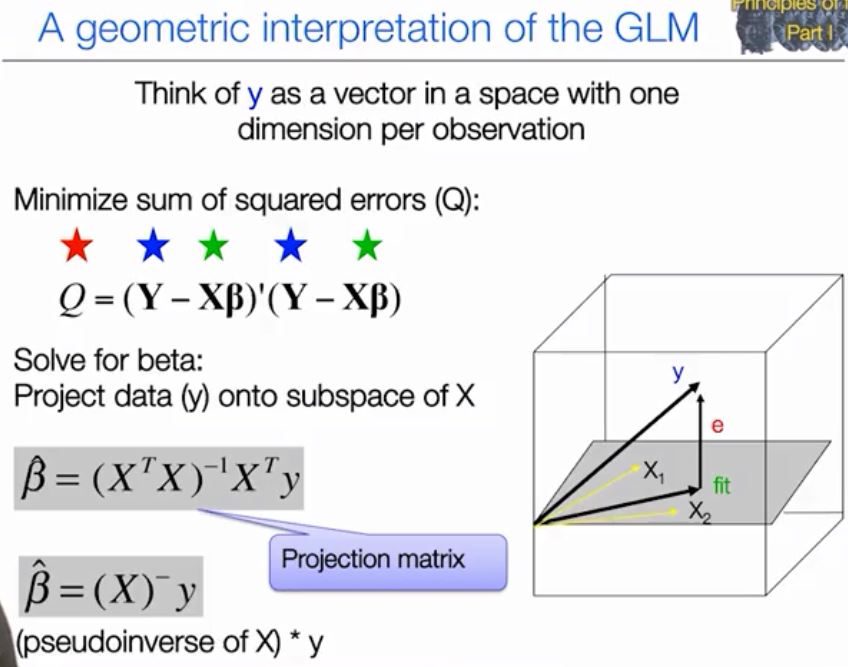
- Interesting angles about GLM
.. When fitting the GLM model, we are actually calculating in a p-dimention hyperplane space (p is the number of independent variables, namely the columns of the design matrix (-1? for the baseline));
.. As the figure shows below, the fitting of the dependent variable y' is actually the projection of y onto the plane that independent variable matrix (design matrix) X defines.
Part 7 - Multiple comparison correction
- voxel-based correction:
FWE (Bonferroni correction & Random Field Theory (usually gaussian random field) & Permutation) - too stringent;
FDR;
- cluster-level inference (correction): sensitivity but bad spacial specifity;
- threshold-free cluster enhancement (TFCE).