分类
为了尝试分类,一种方法是使用线性回归,并将大于0.5的所有预测映射为1,全部小于0.5作为0.然而,该方法不能很好地进行,因为分类实际上不是线性函数。
分类问题就像回归问题一样,只是我们现在想要预测的值只有少量的离散值。现在,我们将重点介绍二进制分类问题,其中y只能取两个值0和1.(我们所说的大部分内容也将归结为多类的情况)。例如,如果我们正在尝试为电子邮件构建垃圾邮件分类器,那么x(i)可能是一个电子邮件的一些功能,如果它是一个垃圾邮件,y可能为1,否则为0。因此,y∈{0,1}。 0也称为负类,1为正类,有时也由符号“ - ”和“+”表示。给定x(i),相应的y(i)也称为培训实例。
Hypothesis Representation
We could approach the classification problem ignoring the fact that y is discrete-valued, and use our old linear regression algorithm to try to predict y given x. However, it is easy to construct examples where this method performs very poorly. Intuitively, it also doesn’t make sense for hθ(x) to take values larger than 1 or smaller than 0 when we know that y ∈ {0, 1}. To fix this, let’s change the form for our hypotheses hθ(x) to satisfy 0≤hθ(x)≤1. This is accomplished by plugging θTx into the Logistic Function.
Our new form uses the "Sigmoid Function," also called the "Logistic Function":
| hθ(x)=g(θTx)z=θTxg(z)=11+e−z |
The following image shows us what the sigmoid function looks like:

The function g(z), shown here, maps any real number to the (0, 1) interval, making it useful for transforming an arbitrary-valued function into a function better suited for classification.
hθ(x) will give us the probability that our output is 1. For example, hθ(x)=0.7 gives us a probability of 70% that our output is 1. Our probability that our prediction is 0 is just the complement of our probability that it is 1 (e.g. if probability that it is 1 is 70%, then the probability that it is 0 is 30%).
| hθ(x)=P(y=1|x;θ)=1−P(y=0|x;θ)P(y=0|x;θ)+P(y=1|x;θ)=1 |
Decision Boundary
In order to get our discrete 0 or 1 classification, we can translate the output of the hypothesis function as follows:
| hθ(x)≥0.5→y=1hθ(x)<0.5→y=0 |
The way our logistic function g behaves is that when its input is greater than or equal to zero, its output is greater than or equal to 0.5:
| g(z)≥0.5whenz≥0 |
Remember.
| z=0,e0=1⇒g(z)=1/2z→∞,e−∞→0⇒g(z)=1z→−∞,e∞→∞⇒g(z)=0 |
So if our input to g is θTX, then that means:
| hθ(x)=g(θTx)≥0.5whenθTx≥0 |
From these statements we can now say:
| θTx≥0⇒y=1θTx<0⇒y=0 |
The decision boundary is the line that separates the area where y = 0 and where y = 1. It is created by our hypothesis function.
Example:
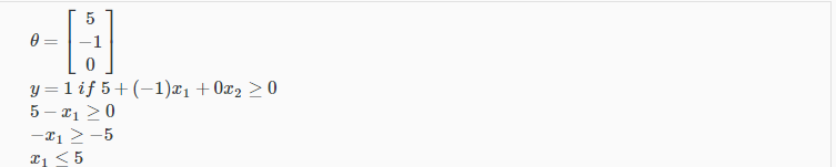
Again, the input to the sigmoid function g(z) (e.g. θTX) doesn't need to be linear, and could be a function that describes a circle (e.g. z=θ0+θ1x21+θ2x22) or any shape to fit our data.In this case, our decision boundary is a straight vertical line placed on the graph where x1=5, and everything to the left of that denotes y = 1, while everything to the right denotes y = 0.