1首先是sklearn的官网:http://scikit-learn.org/stable/
在官网网址上可以看到很多的demo,下边这张是一张非常有用的流程图,在这个流程图中,可以根据数据集的特征,选择合适的方法。

2.sklearn使用的小例子
import numpy as np
from sklearn import datasets
from sklearn.cross_validation import train_test_split
from sklearn.neighbors import KNeighborsClassifier

iris=datasets.load_iris()
iris_X=iris.data
iris_y=iris.target

print(iris_X[:2,:])    #输出数据的前2行,
print(iris_y)

X_train,X_test,y_train,y_test=train_test_split(iris_X,iris_y,test_size=0.3)    #把数据集分为训练集和测试集两个部分一部分是训练集,一部分是测试集,其中测试集占了30%
print(y_train)

knn=KNeighborsClassifier()
knn.fit(X_train,y_train)
print(knn.predict(X_test))
print(y_test)
3.sklearn数据集
在上边例子中,直接使用了sklearn的数据集,在这个包中还有很多其他的数据集,数据集的网址:http://scikit-learn.org/stable/modules/classes.html#module-sklearn.datasets不仅可以使用数据集中的数据,还可以生成虚拟的数据,
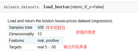
sklearn中自带的数据集,以房屋数据集为例:
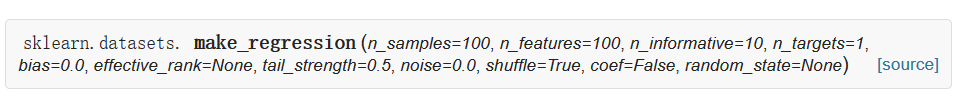
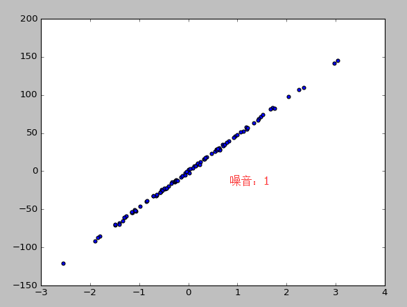
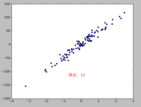
sklearn可以生成的数据集,回归模型中使用的数据集为例:
| Parameters: |
n_samples : int, optional (default=100):The number of samples. n_features : int, optional (default=100):The number of features. n_informative : int, optional (default=10):The number of informative features, i.e., the number of features used to build the linear model used to generate the output. n_targets : int, optional (default=1):The number of regression targets, i.e., the dimension of the y output vector associated with a sample. By default, the output is a scalar. bias : float, optional (default=0.0):The bias term in the underlying linear model. effective_rank : int or None, optional (default=None) if not None:The approximate number of singular vectors required to explain most of the input data by linear combinations. Using this kind of singular spectrum in the input allows the generator to reproduce the correlations often observed in practice. if None:The input set is well conditioned, centered and gaussian with unit variance. tail_strength : float between 0.0 and 1.0, optional (default=0.5):The relative importance of the fat noisy tail of the singular values profile if effective_rank is not None. noise : float, optional (default=0.0):The standard deviation of the gaussian noise applied to the output. shuffle : boolean, optional (default=True):Shuffle the samples and the features. coef : boolean, optional (default=False):If True, the coefficients of the underlying linear model are returned. random_state : int, RandomState instance or None, optional (default=None):If int, random_state is the seed used by the random number generator; If RandomState instance, random_state is the random number generator; If None, the random number generator is the RandomState instance used by np.random. |
|---|---|
| Returns: |
X : array of shape [n_samples, n_features]:The input samples. y : array of shape [n_samples] or [n_samples, n_targets]:The output values. coef : array of shape [n_features] or [n_features, n_targets], optional:The coefficient of the underlying linear model. It is returned only if coef is True. |
from sklearn import datasets
from sklearn.linear_model import LinearRegression
import matplotlib.pyplot as plt

#使用以后的数据集进行线性回归
loaded_data=datasets.load_boston()
data_X=loaded_data.data
data_y=loaded_data.target

model=LinearRegression()
model.fit(data_X,data_y)

print(model.predict(data_X[:4,:]))
print(data_y[:4])

#使用生成线性回归的数据集,最后的数据集结果用散点图表示
X,y=datasets.make_regression(n_samples=100,n_features=1,n_targets=1,noise=10)   #n_samples表示样本数目,n_features特征的数目  n_tragets  noise噪音
plt.scatter(X,y)
plt.show()
4。模型的参数
sklearn 的 model 属性和功能都是高度统一的. 你可以运用到这些属性查看 model 的参数和值等等.
from sklearn import datasets
from sklearn.linear_model import LinearRegression
import matplotlib.pyplot as plt

#使用以后的数据集进行线性回归
loaded_data=datasets.load_boston()
data_X=loaded_data.data
data_y=loaded_data.target

model=LinearRegression()
model.fit(data_X,data_y)

print(model.predict(data_X[:4,:]))
print(data_y[:4])

#参数
print(model.coef_)      #如果y=0.1x+0.3   则此行输出的结果为0.1
print(model.intercept_)             #此行输出的结果为0.3
print(model.get_params())       #模型定义时定义的参数,如果没有定义则返回默认值
print(model.score(data_X,data_y))   #给训练模型打分,注意用在LinearR中使用R^2 conefficient of determination打分
输出的结果:
[ 30.00821269  25.0298606   30.5702317   28.60814055]
[ 24.   21.6  34.7  33.4]
[ -1.07170557e-01   4.63952195e-02   2.08602395e-02   2.68856140e+00
  -1.77957587e+01   3.80475246e+00   7.51061703e-04  -1.47575880e+00
   3.05655038e-01  -1.23293463e-02  -9.53463555e-01   9.39251272e-03
  -5.25466633e-01]
36.4911032804
{'fit_intercept': True, 'normalize': False, 'n_jobs': 1, 'copy_X': True}
0.740607742865
5.标准化:normalization
normalization 在数据跨度不一的情况下对机器学习有很重要的作用.特别是各种数据属性还会互相影响的情况之下. Scikit-learn 中标准化的语句是 preprocessing.scale() . scale 以后, model 就更能从标准化数据中学到东西.
from sklearn import preprocessing #进行标准化数据时,需要引入个包
import numpy as np
from sklearn.cross_validation import train_test_split
from sklearn.datasets.samples_generator import  make_classification
from sklearn.svm import SVC
import matplotlib.pyplot as plt


X,y=make_classification(n_samples=300,n_features=2,n_redundant=0,n_informative=2,random_state=22,n_clusters_per_class=1,scale=100)

#X=preprocessing.minmax_scale(X,feature_range=(-1,1))
X=preprocessing.scale(X)   #0.966666666667 没有 0.477777777778
X_train,X_test,y_train,y_test=train_test_split(X,y,test_size=0.3)
clf=SVC()
clf.fit(X_train,y_train)
print(clf.score(X_test,y_test))


plt.scatter(X[:,0],X[:,1],c=y)
plt.show()

a=np.array([[10,2.7,3.6],
            [-100,5,-2],
            [120,20,40]],dtype=np.float64)   #每一列代表一个属性
print(a)       #标准化之前a
print(preprocessing.scale(a)) #标准化之后的a
6.交叉验证 cross validation(1)
sklearn 中的 cross validation 交叉验证 对于我们选择正确的 model 和model 的参数是非常有帮助的. 有了他的帮助, 我们能直观的看出不同 model 或者参数对结构准确度的影响.
from sklearn.datasets import load_iris
from sklearn.cross_validation import train_test_split
from sklearn.neighbors import KNeighborsClassifier

iris=load_iris()
iris_X=iris.data
iris_y=iris.target

#直接训练
X_train,X_test,y_train,y_test=train_test_split(iris_X,iris_y,random_state=4)    #把数据集分为训练集和测试集两个部分一部分是训练集,一部分是测试集,其中测试集占了30%
knn=KNeighborsClassifier(n_neighbors=5)
knn.fit(X_train,y_train)
print(knn.score(X_test,y_test))   #0.973684210526

#交叉验证
from sklearn.cross_validation import cross_val_score
knn=KNeighborsClassifier(n_neighbors=5)
score=cross_val_score(knn,iris_X,iris_y,cv=5,scoring='accuracy')  #c分成几组 scoring是准确度
print(score)
print(score.mean())

import matplotlib.pyplot as plt
k_range=range(1,31)
k_score=[]
for k in k_range:
    knn=KNeighborsClassifier(n_neighbors=k)
    #score=cross_val_score(knn,iris_X,iris_y,cv=10,scoring='accuracy')#for classification   精度
    loss=-cross_val_score(knn,iris_X,iris_y,cv=10,scoring='mean_squared_error') #for regression    损失函数
    #k_score.append(score.mean())
    k_score.append(loss.mean())
plt.plot(k_range,k_score)
plt.xlabel("Value of K for KNN")
plt.ylabel("Cross-validates Accuracy")
plt.show()
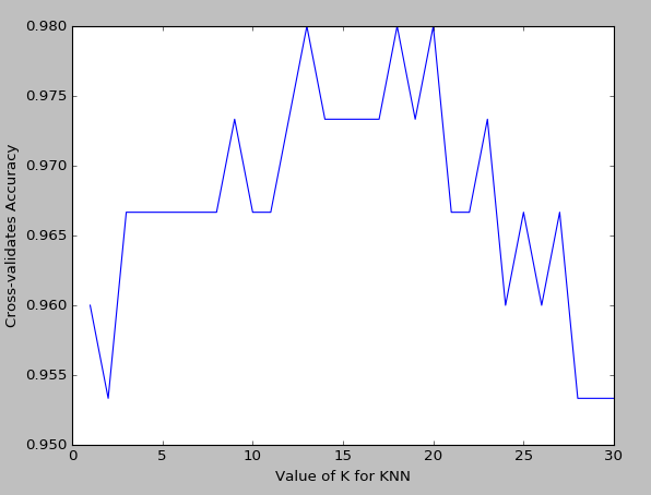
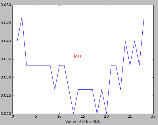
k越大越容易underfitting而不是overfitting
如果想要对不同的机器学习模型来计算,可能需要把knn的值换一下
7.交叉验证 cross validation(2)
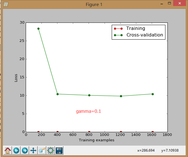
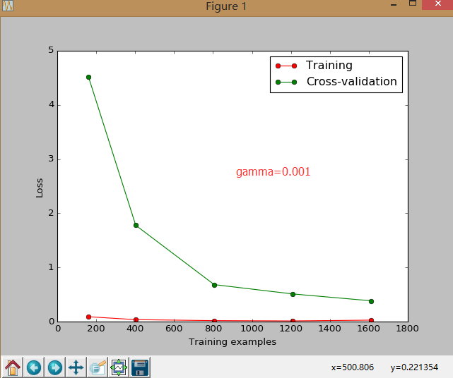
sklearn.learning_curve 中的 learning curve 可以很直观的看出我们的 model 学习的进度,对比发现有没有 overfitting 的问题.然后我们可以对我们的 model 进行调整,克服 overfitting 的问题.
from sklearn.learning_curve import learning_curve   #可视化学习的整个过程
from sklearn.datasets import load_digits
from sklearn.svm import SVC
import matplotlib.pyplot as plt
import numpy as np

digits=load_digits()
X=digits.data
y=digits.target
train_sizes,train_loss,test_loss=learning_curve(
    SVC(gamma=0.1),X,y,cv=10,scoring="mean_squared_error",
    train_sizes=[0.1,0.25,0.5,0.75,1]) #记录的点是学习过程中的10%,25%等等的点
train_loss_mean= (-1)*np.mean(train_loss,axis=1)
test_loss_mean= (-1)*np.mean(test_loss,axis=1)

plt.plot(train_sizes,train_loss_mean,"o-",color="r",label="Training")
plt.plot(train_sizes,test_loss_mean,"o-",color="g",label="Cross-validation")

plt.xlabel("Training examples")
plt.ylabel("Loss")
plt.legend(loc="best")
plt.show()
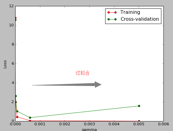
8.交叉验证 cross validation(3)
连续三节的 cross validation让我们知道在机器学习中 validation 是有多么的重要, 这一次的 sklearn 中我们用到了 sklearn.learning_curve 当中的另外一种, 叫做 validation_curve, 用这一种 curve 我们就能更加直观看出改变 model 中的参数的时候有没有 overfitting 的问题了.这也是可以让我们更好的选择参数的方法.
from sklearn.learning_curve import validation_curve   #可视化学习的整个过程
from sklearn.datasets import load_digits
from sklearn.svm import SVC
import matplotlib.pyplot as plt
import numpy as np

digits=load_digits()
X=digits.data
y=digits.target
gamma_range=np.logspace(-6,-2.3,5)#从-6到-2.3取5个点
train_loss,test_loss=validation_curve(
    SVC(),X,y,param_name="gamma",param_range=gamma_range,cv=10,scoring="mean_squared_error")
train_loss_mean= (-1)*np.mean(train_loss,axis=1)
test_loss_mean= (-1)*np.mean(test_loss,axis=1)

plt.plot(gamma_range,train_loss_mean,"o-",color="r",label="Training")
plt.plot(gamma_range,test_loss_mean,"o-",color="g",label="Cross-validation")

plt.xlabel("gamma")
plt.ylabel("Loss")
plt.legend(loc="best")
plt.show()
9,存储模型:
我们练习好了一个 model 以后总需要保存和再次预测, 所以保存和读取我们的 sklearn model 也是同样重要的一步.本文采用了两种方法来存储
from sklearn import svm
from sklearn import datasets

clf=svm.SVC()
iris=datasets.load_iris()
X,y=iris.data,iris.target
clf.fit(X,y)

#method1:pickle
import pickle
#save
with open('save/clf.pickle','wb')as f:
    pickle.dump(clf,f)

#restore
with open('save/clf.pickle','rb') as f:
    clf=pickle.load(f)
    print(clf.predict(X[0:1]))


#method2:joblib
from sklearn.externals import joblib
#save
joblib.dump(clf,'save/clf.pkl')
clf3=joblib.load('save/clf.pkl')
print(clf3.predict(X[0:1]))
youtube学习 :
周莫烦:https://www.youtube.com/user/MorvanZhou
个人主页:https://morvanzhou.github.io/tutorials/
源码:https://github.com/MorvanZhou