一种新型聚类算法(Clustering by fast search and find of density peaksd)

最近在学习论文的时候发现了在science上发表的关于新型的基于密度的聚类算法

Kmean算法有很多不足的地方，比如k值的确定，初始结点选择，而且还不能检测费球面类别的数据分布，对于第二个问题，提出了Kmean++，而其他不足还没有解决，dbscan虽然可以对任意形状分布的进行聚类，但是必须指定一个密度阈值，从而去除低于此密度阈值的噪音点，这篇文章解决了这些不足。

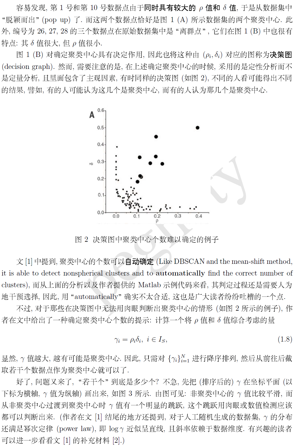
本文提出的聚类算法的核心思想在于，对聚类中心的刻画上，而且认为聚类中心同时具有以下两种特点：

• 本身的密度大，即它被密度均不超过它的邻居包围
• 与其他密度更大的数据点之间的“距离”相对更大

 

通俗的理解为：给一个节点求与其距离小于一个值的节点的个数，用这个个数表示节点的密度，此时求出来的就是节点的局部密度，

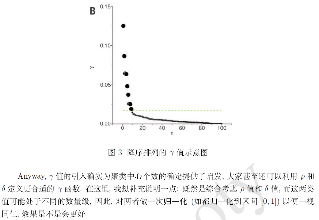
经过上边的过程，每个点都可以找到两个距离与之对应，然后建立一个二维坐标轴，在坐标轴上把图形画出来，如下图

 

最后，附上作者在补充材料里提供的 Matlab 示例程序 （加了适当的代码注释）

clear all  
close all  
disp('The only input needed is a distance matrix file')  
disp('The format of this file should be: ')  
disp('Column 1: id of element i')  
disp('Column 2: id of element j')  
disp('Column 3: dist(i,j)')  
  
%% 从文件中读取数据  
mdist=input('name of the distance matrix file (with single quotes)?
');  
disp('Reading input distance matrix')  
xx=load(mdist);  
ND=max(xx(:,2));  
NL=max(xx(:,1));  
if (NL>ND)  
  ND=NL;  %% 确保 DN 取为第一二列最大值中的较大者，并将其作为数据点总数  
end  
  
N=size(xx,1); %% xx 第一个维度的长度，相当于文件的行数（即距离的总个数）  
  
%% 初始化为零  
for i=1:ND  
  for j=1:ND  
    dist(i,j)=0;  
  end  
end  
  
%% 利用 xx 为 dist 数组赋值，注意输入只存了 0.5*DN(DN-1) 个值，这里将其补成了满矩阵  
%% 这里不考虑对角线元素  
for i=1:N  
  ii=xx(i,1);  
  jj=xx(i,2);  
  dist(ii,jj)=xx(i,3);  
  dist(jj,ii)=xx(i,3);  
end  
  
%% 确定 dc  
  
percent=2.0;  
fprintf('average percentage of neighbours (hard coded): %5.6f
', percent);  
  
position=round(N*percent/100); %% round 是一个四舍五入函数  
sda=sort(xx(:,3)); %% 对所有距离值作升序排列  
dc=sda(position);  
  
%% 计算局部密度 rho (利用 Gaussian 核)  
  
fprintf('Computing Rho with gaussian kernel of radius: %12.6f
', dc);  
  
%% 将每个数据点的 rho 值初始化为零  
for i=1:ND  
  rho(i)=0.;  
end  
  
% Gaussian kernel  
for i=1:ND-1  
  for j=i+1:ND  
     rho(i)=rho(i)+exp(-(dist(i,j)/dc)*(dist(i,j)/dc));  
     rho(j)=rho(j)+exp(-(dist(i,j)/dc)*(dist(i,j)/dc));  
  end  
end  
  
% "Cut off" kernel  
%for i=1:ND-1  
%  for j=i+1:ND  
%    if (dist(i,j)<dc)  
%       rho(i)=rho(i)+1.;  
%       rho(j)=rho(j)+1.;  
%    end  
%  end  
%end  
  
%% 先求矩阵列最大值，再求最大值，最后得到所有距离值中的最大值  
maxd=max(max(dist));   
  
%% 将 rho 按降序排列，ordrho 保持序  
[rho_sorted,ordrho]=sort(rho,'descend');  
   
%% 处理 rho 值最大的数据点  
delta(ordrho(1))=-1.;  
nneigh(ordrho(1))=0;  
  
%% 生成 delta 和 nneigh 数组  
for ii=2:ND  
   delta(ordrho(ii))=maxd;  
   for jj=1:ii-1  
     if(dist(ordrho(ii),ordrho(jj))<delta(ordrho(ii)))  
        delta(ordrho(ii))=dist(ordrho(ii),ordrho(jj));  
        nneigh(ordrho(ii))=ordrho(jj);   
        %% 记录 rho 值更大的数据点中与 ordrho(ii) 距离最近的点的编号 ordrho(jj)  
     end  
   end  
end  
  
%% 生成 rho 值最大数据点的 delta 值  
delta(ordrho(1))=max(delta(:));  
  
%% 决策图  
  
disp('Generated file:DECISION GRAPH')   
disp('column 1:Density')  
disp('column 2:Delta')  
  
fid = fopen('DECISION_GRAPH', 'w');  
for i=1:ND  
   fprintf(fid, '%6.2f %6.2f
', rho(i),delta(i));  
end  
  
%% 选择一个围住类中心的矩形  
disp('Select a rectangle enclosing cluster centers')  
  
%% 每台计算机，句柄的根对象只有一个，就是屏幕，它的句柄总是 0  
%% >> scrsz = get(0,'ScreenSize')  
%% scrsz =  
%%            1           1        1280         800  
%% 1280 和 800 就是你设置的计算机的分辨率，scrsz(4) 就是 800，scrsz(3) 就是 1280  
scrsz = get(0,'ScreenSize');  
  
%% 人为指定一个位置，感觉就没有那么 auto 了 :-)  
figure('Position',[6 72 scrsz(3)/4. scrsz(4)/1.3]);  
  
%% ind 和 gamma 在后面并没有用到  
for i=1:ND  
  ind(i)=i;   
  gamma(i)=rho(i)*delta(i);  
end  
  
%% 利用 rho 和 delta 画出一个所谓的“决策图”  
  
subplot(2,1,1)  
tt=plot(rho(:),delta(:),'o','MarkerSize',5,'MarkerFaceColor','k','MarkerEdgeColor','k');  
title ('Decision Graph','FontSize',15.0)  
xlabel ('
ho')  
ylabel ('delta')  
  
subplot(2,1,1)  
rect = getrect(1);   
%% getrect 从图中用鼠标截取一个矩形区域， rect 中存放的是  
%% 矩形左下角的坐标 (x,y) 以及所截矩形的宽度和高度  
rhomin=rect(1);  
deltamin=rect(2); %% 作者承认这是个 error，已由 4 改为 2 了!  
  
%% 初始化 cluster 个数  
NCLUST=0;  
  
%% cl 为归属标志数组，cl(i)=j 表示第 i 号数据点归属于第 j 个 cluster  
%% 先统一将 cl 初始化为 -1  
for i=1:ND  
  cl(i)=-1;  
end  
  
%% 在矩形区域内统计数据点（即聚类中心）的个数  
for i=1:ND  
  if ( (rho(i)>rhomin) && (delta(i)>deltamin))  
     NCLUST=NCLUST+1;  
     cl(i)=NCLUST; %% 第 i 号数据点属于第 NCLUST 个 cluster  
     icl(NCLUST)=i;%% 逆映射,第 NCLUST 个 cluster 的中心为第 i 号数据点  
  end  
end  
  
fprintf('NUMBER OF CLUSTERS: %i 
', NCLUST);  
  
disp('Performing assignation')  
  
%% 将其他数据点归类 (assignation)  
for i=1:ND  
  if (cl(ordrho(i))==-1)  
    cl(ordrho(i))=cl(nneigh(ordrho(i)));  
  end  
end  
%% 由于是按照 rho 值从大到小的顺序遍历,循环结束后, cl 应该都变成正的值了.   
  
%% 处理光晕点，halo这段代码应该移到 if (NCLUST>1) 内去比较好吧  
for i=1:ND  
  halo(i)=cl(i);  
end  
  
if (NCLUST>1)  
  
  % 初始化数组 bord_rho 为 0,每个 cluster 定义一个 bord_rho 值  
  for i=1:NCLUST  
    bord_rho(i)=0.;  
  end  
  
  % 获取每一个 cluster 中平均密度的一个界 bord_rho  
  for i=1:ND-1  
    for j=i+1:ND  
      %% 距离足够小但不属于同一个 cluster 的 i 和 j  
      if ((cl(i)~=cl(j))&& (dist(i,j)<=dc))  
        rho_aver=(rho(i)+rho(j))/2.; %% 取 i,j 两点的平均局部密度  
        if (rho_aver>bord_rho(cl(i)))   
          bord_rho(cl(i))=rho_aver;  
        end  
        if (rho_aver>bord_rho(cl(j)))   
          bord_rho(cl(j))=rho_aver;  
        end  
      end  
    end  
  end  
  
  %% halo 值为 0 表示为 outlier  
  for i=1:ND  
    if (rho(i)<bord_rho(cl(i)))  
      halo(i)=0;  
    end  
  end  
  
end  
  
%% 逐一处理每个 cluster  
for i=1:NCLUST  
  nc=0; %% 用于累计当前 cluster 中数据点的个数  
  nh=0; %% 用于累计当前 cluster 中核心数据点的个数  
  for j=1:ND  
    if (cl(j)==i)   
      nc=nc+1;  
    end  
    if (halo(j)==i)   
      nh=nh+1;  
    end  
  end  
  
  fprintf('CLUSTER: %i CENTER: %i ELEMENTS: %i CORE: %i HALO: %i 
', i,icl(i),nc,nh,nc-nh);  
  
end  
  
cmap=colormap;  
for i=1:NCLUST  
   ic=int8((i*64.)/(NCLUST*1.));  
   subplot(2,1,1)  
   hold on  
   plot(rho(icl(i)),delta(icl(i)),'o','MarkerSize',8,'MarkerFaceColor',cmap(ic,:),'MarkerEdgeColor',cmap(ic,:));  
end  
subplot(2,1,2)  
disp('Performing 2D nonclassical multidimensional scaling')  
Y1 = mdscale(dist, 2, 'criterion','metricstress');  
plot(Y1(:,1),Y1(:,2),'o','MarkerSize',2,'MarkerFaceColor','k','MarkerEdgeColor','k');  
title ('2D Nonclassical multidimensional scaling','FontSize',15.0)  
xlabel ('X')  
ylabel ('Y')  
for i=1:ND  
 A(i,1)=0.;  
 A(i,2)=0.;  
end  
for i=1:NCLUST  
  nn=0;  
  ic=int8((i*64.)/(NCLUST*1.));  
  for j=1:ND  
    if (halo(j)==i)  
      nn=nn+1;  
      A(nn,1)=Y1(j,1);  
      A(nn,2)=Y1(j,2);  
    end  
  end  
  hold on  
  plot(A(1:nn,1),A(1:nn,2),'o','MarkerSize',2,'MarkerFaceColor',cmap(ic,:),'MarkerEdgeColor',cmap(ic,:));  
end  
  
%for i=1:ND  
%   if (halo(i)>0)  
%      ic=int8((halo(i)*64.)/(NCLUST*1.));  
%      hold on  
%      plot(Y1(i,1),Y1(i,2),'o','MarkerSize',2,'MarkerFaceColor',cmap(ic,:),'MarkerEdgeColor',cmap(ic,:));  
%   end  
%end  
faa = fopen('CLUSTER_ASSIGNATION', 'w');  
disp('Generated file:CLUSTER_ASSIGNATION')  
disp('column 1:element id')  
disp('column 2:cluster assignation without halo control')  
disp('column 3:cluster assignation with halo control')  
for i=1:ND  
   fprintf(faa, '%i %i %i
',i,cl(i),halo(i));  
end  

 参考：http://blog.csdn.net/aimatfuture/article/details/39405261

http://blog.csdn.net/zxdxyz/article/details/40655231