（六）6.11 Neurons Networks implements of self-taught learning

在machine learning领域，更多的数据往往强于更优秀的算法，然而现实中的情况是一般人无法获取大量的已标注数据，这时候可以通过无监督方法获取大量的未标注数据，自学习（ self-taught learning）与无监督特征学习（unsupervised feature learning）就是这种算法。虽然同等条件下有标注数据蕴含的信息多于无标注数据，但是若能获取大量的无标注数据并且计算机能够加以利用，计算机往往可以取得比较良好的结果。

通过自学习与无监督特征学习，可以得到大量的无标注数据，学习出较好的特征描述，在尝试解决一个具体的分类问题时，可以基于这些学习出的特征描述和任意的（可能比较少的）已标注数据，使用有监督学习方法在标注数据上完成分类。

在拥有大量未标注数据和少量已标注数据的场景下，通过对所有x⁽ⁱ⁾进行特征学习得到a⁽ⁱ⁾，在标注数据中用a⁽ⁱ⁾替原始的输入x⁽ⁱ⁾得到新的训练样本{a⁽ⁱ⁾  ,y⁽ⁱ⁾ }(i=1...m)，即可取得很好的效果，即使在只有标注数据的情况下，本算法依然能取得很好的效果。

autoencoder可以在无标注数据集中学习特征，给定一个无标注的训练数据集（下标  代表“不带类标”），首先进行预处理，比如pca或者白化，然后训练一个sparse autoencoder:

'

通过训练得到的模型参数 ，给定任意的输入数据 ，可以计算隐藏单元的激活量（activations） 。相比原始输入  来说， 可能是一个更好的特征描述。下图的神经网络描述了特征（激活量 ）的计算：

对应之前所提到的，假定有 个 已标注训练集 （下标  表示“带类标”），现在可以为输入数据找到更好的特征描述。将  输入到稀疏自编码器，得到隐藏单元激活量 。接下来，可以直接使用  来代替原始数据  （“替代表示”,Replacement Representation）。也可以合二为一，使用新的向量  来代替原始数据  （“级联表示”,Concatenation Representation）。

经过变换后，训练集就变成 或者是（取决于使用  替换  还是将二者合并）。在实践中，将  和  合并通常表现的更好。考虑到内存和计算的成本，也可以使用替换操作。

最终，可以训练出一个有监督学习算法（例如 svm, logistic regression 等），得到一个判别函数对  值进行预测。预测过程如下：给定一个测试样本 ，重复之前的过程，将其送入稀疏自编码器，得到 。然后将  （或者  ）送入分类器中，得到预测值。

从未标注训练集  中学习这一过程中可能计算了各种数据预处理参数。例如计算数据均值并且对数据做均值标准化（mean normalization）；或者对原始数据做主成分分析（PCA），然后将原始数据表示为  (又或者使用 PCA 白化或 ZCA 白化)。这样的话，有必要将这些参数保存起来，并且在后面的训练和测试阶段使用同样的参数，以保证新来（测试）数据进入稀疏自编码神经网络之前经过了同样的变换。例如，如果对未标注数据集进行PCA预处理，就必须将得到的矩阵  保存起来，并且应用到有标注训练集和测试集上；而不能使用有标注训练集重新估计出一个不同的矩阵  （也不能重新计算均值并做均值标准化），否则的话可能得到一个完全不一致的数据预处理操作，导致进入自编码器的数据分布迥异于训练自编码器时的数据分布。

有两种常见的无监督特征学习方式，区别在于有什么样的未标注数据。自学习(self-taught learning) 是其中更为一般的、更强大的学习方式，它不要求未标注数据  和已标注数据  来自同样的分布。另外一种带限制性的方式也被称为半监督学习，它要求 和 服从同样的分布。下面通过例子解释二者的区别。

假定有一个计算机视觉方面的任务，目标是区分汽车和摩托车图像；也即训练样本里面要么是汽车的图像，要么是摩托车的图像。哪里可以获取大量的未标注数据呢？最简单的方式可能是从互联网上下载一些随机的图像数据集，在这些数据上训练出一个稀疏自编码器，从中得到有用的特征。这个例子里，未标注数据完全来自于一个和已标注数据不同的分布（未标注数据集中，或许其中一些图像包含汽车或者摩托车，但是不是所有的图像都如此）。这种情形被称为自学习。

相反，如果有大量的未标注图像数据，要么是汽车图像，要么是摩托车图像，仅仅是缺失了类标号（没有标注每张图片到底是汽车还是摩托车）。也可以用这些未标注数据来学习特征。这种方式，即要求未标注样本和带标注样本服从相同的分布，有时候被称为半监督学习。在实践中，常常无法找到满足这种要求的未标注数据（到哪里找到一个每张图像不是汽车就是摩托车，只是丢失了类标号的图像数据库？）因此，自学习在无标注数据集的特征学习中应用更广。

下面通过自学习的方法，整合sparse autoencoder 与 softmax regression 来构建一个手写数字的分类。

算法步骤：

1）把MNIST数据库的数据分为labeled（0-4） 与 unlabeled（5-9），并且把labeled data 分为 test data 与 train data，一半用来测试，一般用来训练

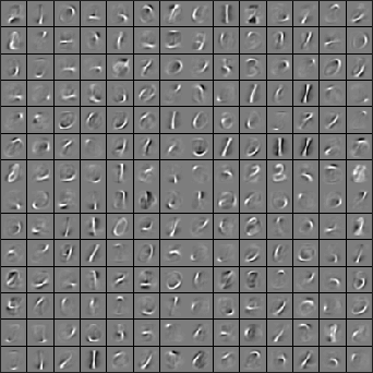
2）用unlabeled data （5-9）训练一个 sparse autoencoder，得到所有参数W⁽¹⁾ W⁽²⁾ b⁽¹⁾ b⁽²⁾ ，记做 θ ，展示第一层参数W⁽¹⁾,展示效果如下：

3）使用上面的sparse autoencoder 训练出来的W⁽¹⁾对labeled data（0-4）训练得到其隐层输出a⁽²⁾，这样不适用原来的像素值，而使用学到的特征来对0-4进行分类。

4）用上述学到的特征a⁽²⁾⁽ⁱ⁾代替原始输入x⁽ⁱ⁾，现在的样本为{(a⁽¹⁾ ,y⁽¹⁾)(a⁽²⁾ ,y⁽²⁾)...(a^(m) ,y^(m))},用该样本来训练我们的softmax分类器。

5）用训练好的softmax进行预测，在labeled data 中的 test data 进行测试即可。准确率讲道理的话应该有98%以上。

一下是matlab代码。部分代码直接调用到之前章节的：

%% CS294A/CS294W Self-taught Learning Exercise

%  Instructions
%  ------------
% 
%  This file contains code that helps you get started on the
%  self-taught learning. You will need to complete code in feedForwardAutoencoder.m
%  You will also need to have implemented sparseAutoencoderCost.m and 
%  softmaxCost.m from previous exercises.
%
%% ======================================================================
%  STEP 0: Here we provide the relevant parameters values that will
%  allow your sparse autoencoder to get good filters; you do not need to 
%  change the parameters below.

inputSize  = 28 * 28;
numLabels  = 5;
hiddenSize = 200;
sparsityParam = 0.1; % desired average activation of the hidden units.
                     % (This was denoted by the Greek alphabet rho, which looks like a lower-case "p",
		             %  in the lecture notes). 
lambda = 3e-3;       % weight decay parameter       
beta = 3;            % weight of sparsity penalty term   
maxIter = 400;

%% ======================================================================
%  STEP 1: Load data from the MNIST database
%
%  This loads our training and test data from the MNIST database files.
%  We have sorted the data for you in this so that you will not have to
%  change it.

% Load MNIST database files
mnistData   = loadMNISTImages('mnist/train-images-idx3-ubyte');
mnistLabels = loadMNISTLabels('mnist/train-labels-idx1-ubyte');

% Set Unlabeled Set (All Images)

% Simulate a Labeled and Unlabeled set
labeledSet   = find(mnistLabels >= 0 & mnistLabels <= 4);
unlabeledSet = find(mnistLabels >= 5);

%把labeled set分为训练数据 和 测试数据
numTrain = round(numel(labeledSet)/2);
trainSet = labeledSet(1:numTrain);
testSet  = labeledSet(numTrain+1:end);

unlabeledData = mnistData(:, unlabeledSet);

trainData   = mnistData(:, trainSet);
trainLabels = mnistLabels(trainSet)' + 1; % Shift Labels 0-4 to the Range 1-5

testData   = mnistData(:, testSet);
testLabels = mnistLabels(testSet)' + 1;   % Shift Labels 0-4 to the Range 1-5

% Output Some Statistics
fprintf('# examples in unlabeled set: %d
', size(unlabeledData, 2));
fprintf('# examples in supervised training set: %d

', size(trainData, 2));
fprintf('# examples in supervised testing set: %d

', size(testData, 2));

%% ======================================================================
%  STEP 2: Train the sparse autoencoder
%  This trains the sparse autoencoder on the unlabeled training
%  images. 

%  Randomly initialize the parameters
theta = initializeParameters(hiddenSize, inputSize);

%% ----------------- YOUR CODE HERE ----------------------
%  Find opttheta by running the sparse autoencoder on
%  unlabeledTrainingImages
%theta 现再是以个展开的向量,对应[W1,W2,b1,b2]的长向量
opttheta = theta; 

opttheta = theta; 
addpath minFunc/
options.Method = 'lbfgs';
options.maxIter = 400;
options.display = 'on';
[opttheta, loss] = minFunc( @(p) sparseAutoencoderLoss(p, ...
      inputSize, hiddenSize, ...
      lambda, sparsityParam, ...
      beta, unlabeledData), ...
      theta, options);


%% -----------------------------------------------------
                          
% Visualize weights，展示W1'（28*28 * 200的矩阵）
% 把该矩阵的每一列展示为一个28*28的图片，来看效果
W1 = reshape(opttheta(1:hiddenSize * inputSize), hiddenSize, inputSize);
display_network(W1');

%%======================================================================
%% STEP 3: Extract Features from the Supervised Dataset
%  
%  You need to complete the code in feedForwardAutoencoder.m so that the 
%  following command will extract features from the data.

trainFeatures = feedForwardAutoencoder(opttheta, hiddenSize, inputSize, ...
                                       trainData);

testFeatures = feedForwardAutoencoder(opttheta, hiddenSize, inputSize, ...
                                       testData);

%%======================================================================
%% STEP 4: Train the softmax classifier

softmaxModel = struct;  
%  Use softmaxTrain.m from the previous exercise to train a multi-class
%  classifier. 

%  Use lambda = 1e-4 for the weight regularization for softmax

% You need to compute softmaxModel using softmaxTrain on trainFeatures and
% trainLabels

lambda = 1e-4;
inputSize = hiddenSize;
numClasses = numel(unique(trainLabels));%unique为找出向量中的非重复元素并进行排序

options.maxIter = 100;
%注意这里的数据不是x^(i)，而是a^(2).
softmaxModel = softmaxTrain(inputSize, numClasses, lambda, ...
                            trainFeatures, trainLabels, options);

%% -----------------------------------------------------


%%======================================================================
%% STEP 5: Testing 

% Compute Predictions on the test set (testFeatures) using softmaxPredict
% and softmaxModel

[pred] = softmaxPredict(softmaxModel, testFeatures);
%% -----------------------------------------------------

% Classification Score
fprintf('Test Accuracy: %f%%
', 100*mean(pred(:) == testLabels(:)));

% (note that we shift the labels by 1, so that digit 0 now corresponds to
%  label 1)
%
% Accuracy is the proportion of correctly classified images
% The results for our implementation was:
%
% Accuracy: 98.3%
%
% 



%%%%%%%%%%%%% 以下对应STEP 3，%%%%%%%%%%%%%%
function [activation] = feedForwardAutoencoder(theta, hiddenSize, visibleSize, data)

% theta: trained weights from the autoencoder
% visibleSize: the number of input units (probably 64) 
% hiddenSize: the number of hidden units (probably 25) 
% data: Our matrix containing the training data as columns.  So, data(:,i) is the i-th training example. 
  
% We first convert theta to the (W1, W2, b1, b2) matrix/vector format, so that this 
% follows the notation convention of the lecture notes. 

W1 = reshape(theta(1:hiddenSize*visibleSize), hiddenSize, visibleSize);
b1 = theta(2*hiddenSize*visibleSize+1:2*hiddenSize*visibleSize+hiddenSize);

%% ---------- YOUR CODE HERE --------------------------------------
%  Instructions: Compute the activation of the hidden layer for the Sparse Autoencoder.
%计算隐层输出a^(2)
activation  = sigmoid(W1*data+repmat(b1,[1,size(data,2)]));

%-------------------------------------------------------------------

end

%-------------------------------------------------------------------
% Here's an implementation of the sigmoid function, which you may find useful
% in your computation of the costs and the gradients.  This inputs a (row or
% column) vector (say (z1, z2, z3)) and returns (f(z1), f(z2), f(z3)). 

function sigm = sigmoid(x)
    sigm = 1 ./ (1 + exp(-x));
end