使用CNN和Python实施的肺炎检测

作者|Muhammad Ardi
编译|Flin
来源|analyticsvidhya

介绍

嘿！几个小时前我刚刚完成一个深度学习项目，现在我想分享一下我所做的事情。这一挑战的目标是确定一个人是否患有肺炎。如果是，则确定是否由细菌或病毒引起。好吧，我觉得这个项目应该叫做分类而不是检测。

换句话说，此任务将是一个多分类问题，其中标签名称为：normal（正常），virus（病毒）和bacteria（细菌）。为了解决这个问题，我将使用CNN（卷积神经网络），它具有出色的图像分类能力，。不仅如此，在这里我还实现了图像增强技术，以提高模型性能。顺便说一句，我获得了80％的测试数据准确性，这对我来说是非常令人印象深刻的。

可以从该Kaggle链接下载此项目中使用的数据集。

• https://www.kaggle.com/paultimothymooney/chest-xray-pneumonia

整个数据集本身的大小约为1 GB，因此下载可能需要一段时间。或者，我们也可以直接创建一个Kaggle Notebook并在那里编码整个项目，因此我们甚至不需要下载任何内容。接下来，如果浏览数据集文件夹，你将看到有3个子文件夹，即train，test和val。

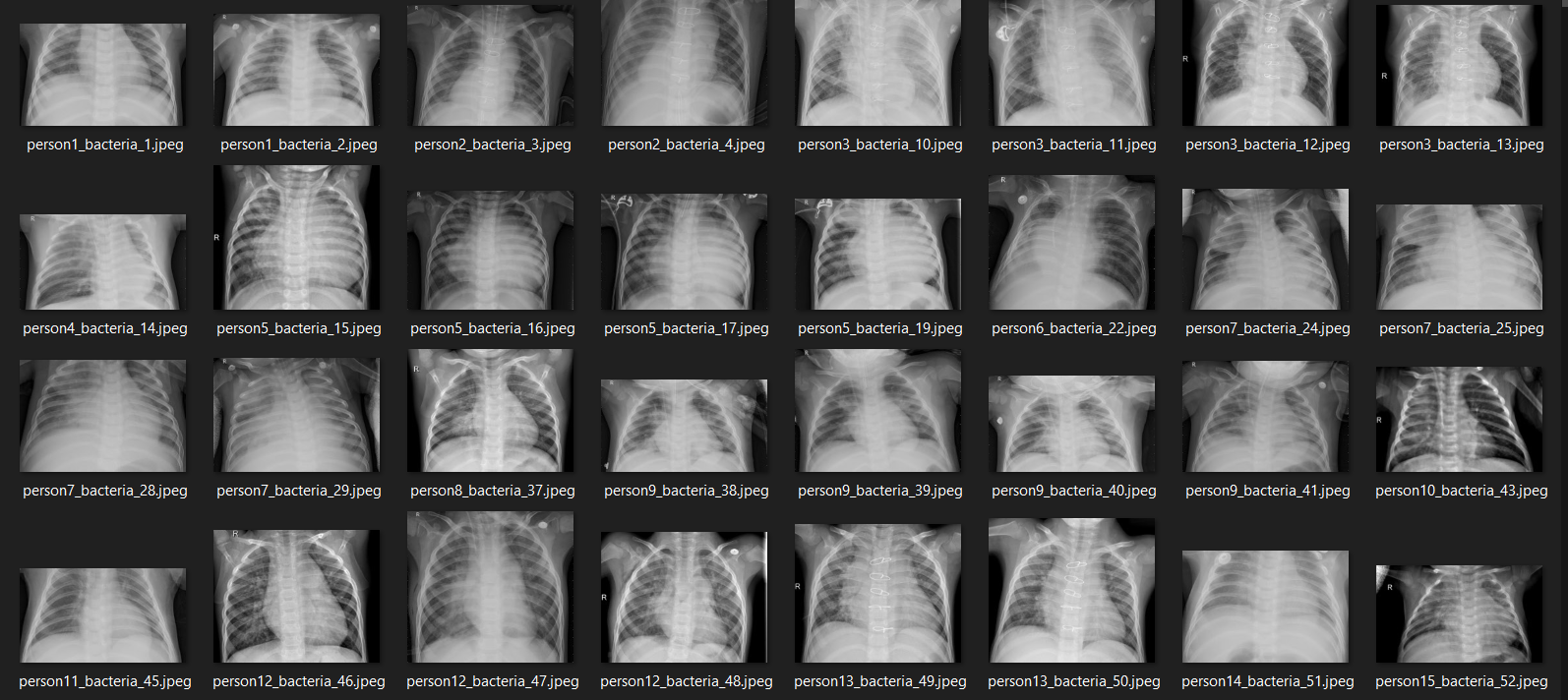
好吧，我认为这些文件夹名称是不言自明的。此外，train文件夹中的数据分别包括正常，病毒和细菌类别的1341、1345和2530个样本。我想这就是我介绍的全部内容了，现在让我们进入代码的编写！

注意：我在本文结尾处放置了该项目中使用的全部代码。

加载模块和训练图像

使用计算机视觉项目时，要做的第一件事是加载所有必需的模块和图像数据本身。我使用tqdm模块显示进度条，稍后你将看到它有用的原因。

我最后导入的是来自Keras模块的ImageDataGenerator。该模块将帮助我们在训练过程中实施图像增强技术。

import os
import cv2
import pickle
import numpy as np
import matplotlib.pyplot as plt
import seaborn as sns
from tqdm import tqdm
from sklearn.preprocessing import OneHotEncoder
from sklearn.metrics import confusion_matrix
from keras.models import Model, load_model
from keras.layers import Dense, Input, Conv2D, MaxPool2D, Flatten
from keras.preprocessing.image import ImageDataGeneratornp.random.seed(22)

接下来，我定义两个函数以从每个文件夹加载图像数据。乍一看，下面的两个功能可能看起来完全一样，但是在使用粗体显示的行上实际上存在一些差异。这样做是因为NORMAL和PNEUMONIA文件夹中的文件名结构略有不同。尽管有所不同，但两个功能执行的其他过程基本相同。

首先，将所有图像调整为200 x 200像素。

这一点很重要，因为所有文件夹中的图像都有不同的尺寸，而神经网络只能接受具有固定数组大小的数据。

接下来，基本上所有图像都存储有3个颜色通道，这对X射线图像来说是多余的。因此，我的想法是将这些彩色图像都转换为灰度图像。

# Do not forget to include the last slash
def load_normal(norm_path):
    norm_files = np.array(os.listdir(norm_path))
    norm_labels = np.array(['normal']*len(norm_files))
    
    norm_images = []
    for image in tqdm(norm_files):
        image = cv2.imread(norm_path + image)
        image = cv2.resize(image, dsize=(200,200))
        image = cv2.cvtColor(image, cv2.COLOR_BGR2GRAY)
        norm_images.append(image)
        
    norm_images = np.array(norm_images)
    
    return norm_images, norm_labels
def load_pneumonia(pneu_path):
    pneu_files = np.array(os.listdir(pneu_path))
    pneu_labels = np.array([pneu_file.split('_')[1] for pneu_file in pneu_files])
    
    pneu_images = []
    for image in tqdm(pneu_files):
        image = cv2.imread(pneu_path + image)
        image = cv2.resize(image, dsize=(200,200))
        image = cv2.cvtColor(image, cv2.COLOR_BGR2GRAY)
        pneu_images.append(image)
        
    pneu_images = np.array(pneu_images)
    
    return pneu_images, pneu_labels

声明了以上两个函数后，现在我们可以使用它来加载训练数据了。如果你运行下面的代码，你还将看到为什么我选择在该项目中实现tqdm模块。

norm_images, norm_labels = load_normal('/kaggle/input/chest-xray-pneumonia/chest_xray/train/NORMAL/')pneu_images, pneu_labels = load_pneumonia('/kaggle/input/chest-xray-pneumonia/chest_xray/train/PNEUMONIA/')

到目前为止，我们已经获得了几个数组：norm_images，norm_labels，pneu_images和pneu_labels。

带_images后缀的表示它包含预处理的图像，而带_labels后缀的数组表示它存储了所有基本信息（也称为标签）。换句话说，norm_images和pneu_images都将成为我们的X数据，其余的将成为y数据。

为了使项目看起来更简单，我将这些数组的值连接起来并存储在X_train和y_train数组中。

X_train = np.append(norm_images, pneu_images, axis=0)
y_train = np.append(norm_labels, pneu_labels)

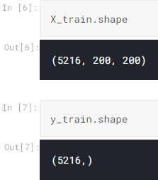
顺便说一句，我使用以下代码获取每个类的图像数：

显示多张图像

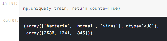
好吧，在这个阶段，显示几个图像并不是强制性的。但我想做是为了确保图片是否已经加载和预处理好。下面的代码用于显示14张从X_train阵列随机拍摄的图像以及标签。

fig, axes = plt.subplots(ncols=7, nrows=2, figsize=(16, 4))

indices = np.random.choice(len(X_train), 14)
counter = 0

for i in range(2):
    for j in range(7):
        axes[i,j].set_title(y_train[indices[counter]])
        axes[i,j].imshow(X_train[indices[counter]], cmap='gray')
        axes[i,j].get_xaxis().set_visible(False)
        axes[i,j].get_yaxis().set_visible(False)
        counter += 1
plt.show()

我们可以看到上图，所有图像现在都具有完全相同的大小，这与我用于本帖子封面图片的图像不同。

加载测试图像

我们已经知道所有训练数据都已成功加载，现在我们可以使用完全相同的函数加载测试数据。步骤几乎相同，但是这里我将那些加载的数据存储在X_test和y_test数组中。用于测试的数据本身包含624个样本。

norm_images_test, norm_labels_test = load_normal('/kaggle/input/chest-xray-pneumonia/chest_xray/test/NORMAL/')pneu_images_test, pneu_labels_test = load_pneumonia('/kaggle/input/chest-xray-pneumonia/chest_xray/test/PNEUMONIA/')X_test = np.append(norm_images_test, pneu_images_test, axis=0)
y_test = np.append(norm_labels_test, pneu_labels_test)

此外，我注意到仅加载整个数据集就需要很长时间。因此，我将使用pickle模块将X_train，X_test，y_train和y_test保存在单独的文件中。这样我下次想再使用这些数据的时候，就不需要再次运行这些代码了。

# Use this to save variables
with open('pneumonia_data.pickle', 'wb') as f:
    pickle.dump((X_train, X_test, y_train, y_test), f)# Use this to load variables
with open('pneumonia_data.pickle', 'rb') as f:
    (X_train, X_test, y_train, y_test) = pickle.load(f)

由于所有X数据都经过了很好的预处理，因此现在使用标签y_train和y_test了。

标签预处理

此时，两个y变量都由以字符串数据类型编写的正常，细菌或病毒组成。实际上，这样的标签只是神经网络所不能接受的。因此，我们需要将其转换为单一格式。

幸运的是，我们从Scikit-Learn模块获取了 OneHotEncoder对象，它对完成转换非常有帮助。为此，我们需要先在y_train和y_test上创建一个新轴。（我们创建了这个新轴，因为那是OneHotEncoder期望的形状）。

y_train = y_train[:, np.newaxis]
y_test = y_test[:, np.newaxis]

接下来，像这样初始化one_hot_encoder。请注意，在这里我将False作为稀疏参数传递，以便简化下一步。但是，如果你想使用稀疏矩阵，则只需使用sparse = True或将参数保留为空即可。

one_hot_encoder = OneHotEncoder(sparse=False)

最后，我们将使用one_hot_encoder将这些y数据转换为one-hot。然后将编码后的标签存储在y_train_one_hot和y_test_one_hot中。这两个数组是我们将用于训练的标签。

y_train_one_hot = one_hot_encoder.fit_transform(y_train)
y_test_one_hot = one_hot_encoder.transform(y_test)

将数据X重塑为（None，200，200，1）

现在让我们回到X_train和X_test。重要的是要知道这两个数组的形状分别为（5216、200、200）和（624、200、200）。

乍一看，这两个形状看起来还可以，因为我们可以使用plt.imshow()函数进行显示。但是，这种形状卷积层不可接受，因为它希望将一个颜色通道作为其输入。

因此，由于该图像本质上是灰度图像，因此我们需要添加一个1维的新轴，该轴将被卷积层识别为唯一的颜色通道。虽然它的实现并不像我的解释那么复杂：

X_train = X_train.reshape(X_train.shape[0], X_train.shape[1], X_train.shape[2], 1)
X_test = X_test.reshape(X_test.shape[0], X_test.shape[1], X_test.shape[2], 1)

运行上述代码后，如果我们同时检查X_train和X_test的形状，那么我们将看到现在的形状分别是（5216，200，200，1）和（624，200，200，1）。

数据扩充

增加数据（或者更具体地说是增加训练数据）的要点是，我们将通过创建更多的样本（每个样本都具有某种随机性）来增加用于训练的数据数量。这些随机性可能包括平移、旋转、缩放、剪切和翻转。

这种技术可以帮助我们的神经网络分类器减少过拟合，或者说，它可以使模型更好地泛化数据样本。幸运的是，由于存在可以从Keras模块导入的ImageDataGenerator对象，实现非常简单。

datagen = ImageDataGenerator(
        rotation_range = 10,  
        zoom_range = 0.1, 
        width_shift_range = 0.1, 
        height_shift_range = 0.1)

因此，我在上面的代码中所做的基本上是设置随机范围。如果你想了解每个参数的详细信息，请点击这里链接到ImageDataGenerator的文档。

• https://keras.io/api/preprocessing/image/

接下来，在初始化datagen对象之后，我们需要做的是使它和我们的X_train相匹配。然后，该过程被随后施加的flow()的方法，该步骤中是非常有用的，使得所述 train_gen对象现在能够产生增强数据的批次。

datagen.fit(X_train)train_gen = datagen.flow(X_train, y_train_one_hot, batch_size=32)

CNN（卷积神经网络）

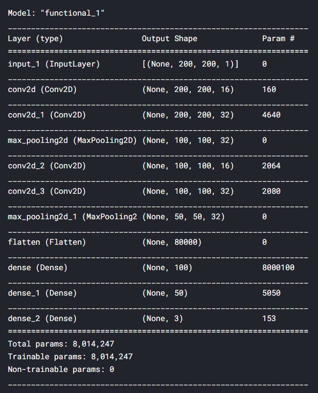
现在是时候真正构建神经网络架构了。让我们从输入层（input1）开始。因此，这一层基本上会获取X数据中的所有图像样本。因此，我们需要确保第一层接受与图像尺寸完全相同的形状。值得注意的是，我们仅需要定义（宽度，高度，通道），而不是（样本，宽度，高度，通道）。

此后，此输入层连接到几对卷积池层对，然后最终连接到全连接层。请注意，由于ReLU的计算速度比S型更快，因此模型中的所有隐藏层都使用ReLU激活函数，因此所需的训练时间更短。最后，要连接的最后一层是output1，它由3个具有softmax激活函数的神经元组成。

这里使用softmax是因为我们希望输出是每个类别的概率值。

input1 = Input(shape=(X_train.shape[1], X_train.shape[2], 1))

cnn = Conv2D(16, (3, 3), activation='relu', strides=(1, 1), 
    padding='same')(input1)
cnn = Conv2D(32, (3, 3), activation='relu', strides=(1, 1), 
    padding='same')(cnn)
cnn = MaxPool2D((2, 2))(cnn)

cnn = Conv2D(16, (2, 2), activation='relu', strides=(1, 1), 
    padding='same')(cnn)
cnn = Conv2D(32, (2, 2), activation='relu', strides=(1, 1), 
    padding='same')(cnn)
cnn = MaxPool2D((2, 2))(cnn)

cnn = Flatten()(cnn)
cnn = Dense(100, activation='relu')(cnn)
cnn = Dense(50, activation='relu')(cnn)
output1 = Dense(3, activation='softmax')(cnn)

model = Model(inputs=input1, outputs=output1)

在使用上面的代码构造了神经网络之后，我们可以通过对model对象应用summary()来显示模型的摘要。下面是我们的CNN模型的详细情况。我们可以看到我们总共有800万个参数——这确实很多。好吧，这就是为什么我在Kaggle Notebook上运行这个代码。

总之，在构建模型之后，我们需要使用分类交叉熵损失函数和Adam优化器来编译神经网络。使用这个损失函数，因为它只是多类分类任务中常用的函数。同时，我选择Adam作为优化器，因为它是在大多数神经网络任务中最小化损失的最佳选择。

model.compile(loss='categorical_crossentropy', 
              optimizer='adam', metrics=['acc'])

现在是时候训练模型了！在这里，我们将使用fit_generator()而不是fit()，因为我们将从train_gen对象获取训练数据。如果你关注数据扩充部分，你会注意到train_gen是使用X_train和y_train_one_hot创建的。因此，我们不需要在fit_generator()方法中显式定义X-y对。

history = model.fit_generator(train_gen, epochs=30, 
          validation_data=(X_test, y_test_one_hot))

train_gen的特殊之处在于，训练过程中将使用具有一定随机性的样本来完成。因此，我们在X_train中拥有的所有训练数据都不会直接输入到神经网络中。取而代之的是，这些样本将被用作生成器的基础，通过一些随机变换生成一个新图像。

此外，该生成器在每个时期产生不同的图像，这对于我们的神经网络分类器更好地泛化测试集中的样本非常有利。下面是训练的过程。

Epoch 1/30
163/163 [==============================] - 19s 114ms/step - loss: 5.7014 - acc: 0.6133 - val_loss: 0.7971 - val_acc: 0.7228
.
.
.
Epoch 10/30
163/163 [==============================] - 18s 111ms/step - loss: 0.5575 - acc: 0.7650 - val_loss: 0.8788 - val_acc: 0.7308
.
.
.
Epoch 20/30
163/163 [==============================] - 17s 102ms/step - loss: 0.5267 - acc: 0.7784 - val_loss: 0.6668 - val_acc: 0.7917
.
.
.
Epoch 30/30
163/163 [==============================] - 17s 104ms/step - loss: 0.4915 - acc: 0.7922 - val_loss: 0.7079 - val_acc: 0.8045

整个训练本身在我的Kaggle Notebook上花费了大约10分钟。所以要耐心点！经过训练后，我们可以绘制出准确度得分的提高和损失值的降低，如下所示：

plt.figure(figsize=(8,6))
plt.title('Accuracy scores')
plt.plot(history.history['acc'])
plt.plot(history.history['val_acc'])
plt.legend(['acc', 'val_acc'])
plt.show()plt.figure(figsize=(8,6))
plt.title('Loss value')
plt.plot(history.history['loss'])
plt.plot(history.history['val_loss'])
plt.legend(['loss', 'val_loss'])
plt.show()

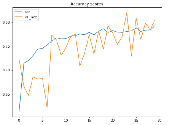
根据上面的两个图，我们可以说，即使在这30个时期内测试准确性和损失值都在波动，模型的性能仍在不断提高。

这里要注意的另一重要事情是，由于我们在项目的早期应用了数据增强方法，因此该模型不会遭受过拟合的困扰。我们在这里可以看到，在最终迭代中，训练和测试数据的准确性分别为79％和80％。

有趣的事实：在实施数据增强方法之前，我在训练数据上获得了100％的准确性，在测试数据上获得了64％的准确性，这显然是过拟合了。因此，我们可以在此处清楚地看到，增加训练数据对于提高测试准确性得分非常有效，同时也可以减少过拟合。

模型评估

现在，让我们深入了解使用混淆矩阵得出的测试数据的准确性。首先，我们需要预测所有X_test并将结果从独热格式转换回其实际的分类标签。

predictions = model.predict(X_test)
predictions = one_hot_encoder.inverse_transform(predictions)

接下来，我们可以像这样使用confusion_matrix()函数：

cm = confusion_matrix(y_test, predictions)

重要的是要注意函数中使用的参数是（实际值，预测值）。该混淆矩阵函数的返回值是一个二维数组，用于存储预测分布。为了使矩阵更易于解释，我们可以使用Seaborn模块中的heatmap()函数进行显示。顺便说一句，这里的类名列表的值是根据one_hot_encoder.categories_返回的顺序获取的。

classnames = ['bacteria', 'normal', 'virus']plt.figure(figsize=(8,8))
plt.title('Confusion matrix')
sns.heatmap(cm, cbar=False, xticklabels=classnames, yticklabels=classnames, fmt='d', annot=True, cmap=plt.cm.Blues)
plt.xlabel('Predicted')
plt.ylabel('Actual')
plt.show()

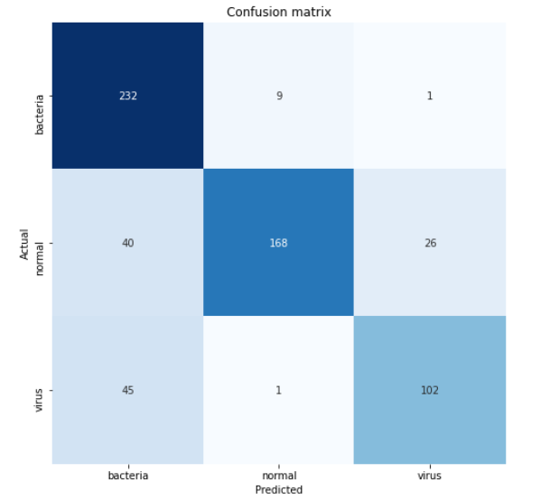
根据上面的混淆矩阵，我们可以看到45张病毒X射线图像被预测为细菌。这可能是因为很难区分这两种肺炎。但是，至少因为我们对242个样本中的232个进行了正确分类，所以我们的模型至少能够很好地预测由细菌引起的肺炎。

这就是整个项目！谢谢阅读！下面是运行整个项目所需的所有代码。

import os
import cv2
import pickle	# Used to save variables
import numpy as np
import matplotlib.pyplot as plt
import seaborn as sns
from tqdm import tqdm	# Used to display progress bar
from sklearn.preprocessing import OneHotEncoder
from sklearn.metrics import confusion_matrix
from keras.models import Model, load_model
from keras.layers import Dense, Input, Conv2D, MaxPool2D, Flatten
from keras.preprocessing.image import ImageDataGenerator	# Used to generate images

np.random.seed(22)

# Do not forget to include the last slash
def load_normal(norm_path):
    norm_files = np.array(os.listdir(norm_path))
    norm_labels = np.array(['normal']*len(norm_files))
    
    norm_images = []
    for image in tqdm(norm_files):
		# Read image
        image = cv2.imread(norm_path + image)
		# Resize image to 200x200 px
        image = cv2.resize(image, dsize=(200,200))
		# Convert to grayscale
        image = cv2.cvtColor(image, cv2.COLOR_BGR2GRAY)
        norm_images.append(image)
        
    norm_images = np.array(norm_images)
    
    return norm_images, norm_labels

def load_pneumonia(pneu_path):
    pneu_files = np.array(os.listdir(pneu_path))
    pneu_labels = np.array([pneu_file.split('_')[1] for pneu_file in pneu_files])
    
    pneu_images = []
    for image in tqdm(pneu_files):
		# Read image
        image = cv2.imread(pneu_path + image)
		# Resize image to 200x200 px
        image = cv2.resize(image, dsize=(200,200))
		# Convert to grayscale
        image = cv2.cvtColor(image, cv2.COLOR_BGR2GRAY)
        pneu_images.append(image)
        
    pneu_images = np.array(pneu_images)
    
    return pneu_images, pneu_labels


print('Loading images')
# All images are stored in _images, all labels are in _labels
norm_images, norm_labels = load_normal('/kaggle/input/chest-xray-pneumonia/chest_xray/train/NORMAL/')
pneu_images, pneu_labels = load_pneumonia('/kaggle/input/chest-xray-pneumonia/chest_xray/train/PNEUMONIA/')

# Put all train images to X_train 
X_train = np.append(norm_images, pneu_images, axis=0)

# Put all train labels to y_train
y_train = np.append(norm_labels, pneu_labels)

print(X_train.shape)
print(y_train.shape)
# Finding out the number of samples of each class
print(np.unique(y_train, return_counts=True))

print('Display several images')
fig, axes = plt.subplots(ncols=7, nrows=2, figsize=(16, 4))

indices = np.random.choice(len(X_train), 14)
counter = 0

for i in range(2):
    for j in range(7):
        axes[i,j].set_title(y_train[indices[counter]])
        axes[i,j].imshow(X_train[indices[counter]], cmap='gray')
        axes[i,j].get_xaxis().set_visible(False)
        axes[i,j].get_yaxis().set_visible(False)
        counter += 1
plt.show()


print('Loading test images')
# Do the exact same thing as what we have done on train data
norm_images_test, norm_labels_test = load_normal('/kaggle/input/chest-xray-pneumonia/chest_xray/test/NORMAL/')
pneu_images_test, pneu_labels_test = load_pneumonia('/kaggle/input/chest-xray-pneumonia/chest_xray/test/PNEUMONIA/')
X_test = np.append(norm_images_test, pneu_images_test, axis=0)
y_test = np.append(norm_labels_test, pneu_labels_test)

# Save the loaded images to pickle file for future use
with open('pneumonia_data.pickle', 'wb') as f:
    pickle.dump((X_train, X_test, y_train, y_test), f)

# Here's how to load it
with open('pneumonia_data.pickle', 'rb') as f:
    (X_train, X_test, y_train, y_test) = pickle.load(f)

print('Label preprocessing')

# Create new axis on all y data
y_train = y_train[:, np.newaxis]
y_test = y_test[:, np.newaxis]

# Initialize OneHotEncoder object
one_hot_encoder = OneHotEncoder(sparse=False)

# Convert all labels to one-hot
y_train_one_hot = one_hot_encoder.fit_transform(y_train)
y_test_one_hot = one_hot_encoder.transform(y_test)

print('Reshaping X data')
# Reshape the data into (no of samples, height, width, 1), where 1 represents a single color channel
X_train = X_train.reshape(X_train.shape[0], X_train.shape[1], X_train.shape[2], 1)
X_test = X_test.reshape(X_test.shape[0], X_test.shape[1], X_test.shape[2], 1)

print('Data augmentation')
# Generate new images with some randomness
datagen = ImageDataGenerator(
		rotation_range = 10,  
        zoom_range = 0.1, 
        width_shift_range = 0.1, 
        height_shift_range = 0.1)

datagen.fit(X_train)
train_gen = datagen.flow(X_train, y_train_one_hot, batch_size = 32)

print('CNN')

# Define the input shape of the neural network
input_shape = (X_train.shape[1], X_train.shape[2], 1)
print(input_shape)

input1 = Input(shape=input_shape)

cnn = Conv2D(16, (3, 3), activation='relu', strides=(1, 1), 
    padding='same')(input1)
cnn = Conv2D(32, (3, 3), activation='relu', strides=(1, 1), 
    padding='same')(cnn)
cnn = MaxPool2D((2, 2))(cnn)

cnn = Conv2D(16, (2, 2), activation='relu', strides=(1, 1), 
    padding='same')(cnn)
cnn = Conv2D(32, (2, 2), activation='relu', strides=(1, 1), 
    padding='same')(cnn)
cnn = MaxPool2D((2, 2))(cnn)

cnn = Flatten()(cnn)
cnn = Dense(100, activation='relu')(cnn)
cnn = Dense(50, activation='relu')(cnn)
output1 = Dense(3, activation='softmax')(cnn)

model = Model(inputs=input1, outputs=output1)

model.compile(loss='categorical_crossentropy', 
              optimizer='adam', metrics=['acc'])

# Using fit_generator() instead of fit() because we are going to use data
# taken from the generator. Note that the randomness is changing
# on each epoch
history = model.fit_generator(train_gen, epochs=30, 
          validation_data=(X_test, y_test_one_hot))

# Saving model
model.save('pneumonia_cnn.h5')

print('Displaying accuracy')
plt.figure(figsize=(8,6))
plt.title('Accuracy scores')
plt.plot(history.history['acc'])
plt.plot(history.history['val_acc'])
plt.legend(['acc', 'val_acc'])
plt.show()

print('Displaying loss')
plt.figure(figsize=(8,6))
plt.title('Loss value')
plt.plot(history.history['loss'])
plt.plot(history.history['val_loss'])
plt.legend(['loss', 'val_loss'])
plt.show()

# Predicting test data
predictions = model.predict(X_test)
print(predictions)

predictions = one_hot_encoder.inverse_transform(predictions)

print('Model evaluation')
print(one_hot_encoder.categories_)

classnames = ['bacteria', 'normal', 'virus']

# Display confusion matrix
cm = confusion_matrix(y_test, predictions)
plt.figure(figsize=(8,8))
plt.title('Confusion matrix')
sns.heatmap(cm, cbar=False, xticklabels=classnames, yticklabels=classnames, fmt='d', annot=True, cmap=plt.cm.Blues)
plt.xlabel('Predicted')
plt.ylabel('Actual')
plt.show()

参考文献

JędrzejDudzicz对胸部X线检查的肺炎检出率约为92％

• https://www.kaggle.com/jedrzejdudzicz/pneumonia-detection-on-chest-x-ray-accuracy-92

Kerian ImageDataGenerator和Adrian Rosebrock的数据增强

• https://www.pyimagesearch.com/2019/07/08/keras-imagedatagenerator-and-data-augmentation/

原文链接：https://www.analyticsvidhya.com/blog/2020/09/pneumonia-detection-using-cnn-with-implementation-in-python/

欢迎关注磐创AI博客站：
http://panchuang.net/

sklearn机器学习中文官方文档：
http://sklearn123.com/

欢迎关注磐创博客资源汇总站：
http://docs.panchuang.net/