实现我们分类数字的网络
好,让我们使用随机梯度下降和 MNIST训练数据来写一个程序来学习怎样识别手写数字。 我们用Python (2.7) 来实现。只有 74 行代码!我们需要的第一个东西是 MNIST数据。如果有 github 账号,你可以将这些代码库克隆下来,
git clone https://github.com/mnielsen/neural-networks-and-deep-learning.git
或者你可以到这里 下载。
顺便说一下, 当我先前说到 MNIST 数据集时,我说它被分成 60,000 个训练图片,和 10,000张测试图片。这是官方的说法。实际上,我们准备用不同的分法。 我们将这60,000张图片的MNIST训练数据集分成两部分:一部分有50,000 张图片,我们用这些图片来训练我们的神经网络,另外的10,000 张的图片用来作确认数据集,用来验证识别是否准确。 在这一章节我们不会使用确认数据,在本系列文章的后面,我们会发现它对于计算出怎样设置神经网络的hyper-parameters是很有用的 - 例如学习率等等,我们的学习算法中可能不会直接用到这些hyper-parameters。虽然确认数据不是源MNIST规格的一部分,很多人按这种方式使用MNIST,确认数据的使用在神经网络中是很常见的。当我提到"MNIST" 从现在起,它表示我们的 50,000个图片数据集,而不是原来的 60,000 张图片数据集*早前提到的, MNIST数据集基于NIST收集的两种数据。为了构建MNIST,数据集被NIST 的Yann LeCun, Corinna Cortes和 Christopher J. C. Burges几个人拆开,放进更方便的格式 点击 此链接 查看更多详情。在我数据集中的数据集是以一种容易加载的格式出现的,并且是用Python来处理这些 MNIST 数据。我是从Montreal大学LISA 机器学习实验室 (链接)获得这些特定格式的数据的。
除了MNIST数据,我们还需要一个Python库Numpy,用来做快速线性代数运算。如果你还没安装这个库,你可以到这里下载: here
让我们讲述一下神经网络代码的核心功能,在我给出完整清单前。核心是一个 Network 类,我们用了表现一个神经网络。下面这些代码是用来初始化一个Network对象:
class Network(object):

    def __init__(self, sizes):
        self.num_layers = len(sizes)
        self.sizes = sizes
        self.biases = [np.random.randn(y, 1) for y in sizes[1:]]
        self.weights = [np.random.randn(y, x)
                        for x, y in zip(sizes[:-1], sizes[1:])]
这些代码,列表的 sizes 包含各个层的神经元的数量。例如,如果我们想创建一个第一层有有两个神经元,第二层有3个神经元,最后一层有一个神经元 的 Network对象,我们这样设置:
net = Network([2, 3, 1])
偏移量和权重,用随机数来初始化,使用 Numpy np.random.randn函数来生成 0均值高斯分布 和标准偏差1. 这个初始的随机数是为了给随机梯度下降算法一个开始点。在接下来的章节我们会找到一种更好的方式来初始化权重和偏移量,但现在暂时用随机数。注意网络的初始化代码假定第一层是输入层,省略这些神经元偏移量的设置,因为偏移量只是用来计算下一层网络的输出值。
也要注意偏移量和权重以Numpy数据矩阵的方式存储。因此,例如 net.weights[1]是一个Numpy矩阵用来储存连接第二层和第三层神经网络的权重。(它不是第一次和第二层,因为Python List 是从0开始算起的)。既然 net.weights[1] 是相当冗长的,让我们用矩阵w来代表。它是一个矩阵,wjk是权重 for the连接在第二层的第k个神经元和 在第三层的第j个神经元。 j 和k 指数的排序可能会看起来很奇怪 - 交换j和k指数会更好吗?使用这个排序的好处是它意味着第三层神经元激活变量是:
这个方程有点长,让我一点一点分析。a是一个激活第二层网络的向量。为了获取a′我们用a乘以权重矩阵w加上偏移量b的和。我们用函数σ来算每个wa+b。
以上记住之后,很容易写出代码来计算网络的输出。我先定义S型函数开始:
def sigmoid(z):
    return 1.0/(1.0+np.exp(-z))
注意当输入 z 是一个向量或者 Numpy 数组, Numpy 自动将函数sigmoid 依次应用到数组的每个元素,以向量化的形式。
我们添加一个 feedforward 方法到 Network 类, 给神经网络一个输入 a ,返回对应的输入*。加入输入值 a 是一个 (n, 1)Numpy ndarray,不是一个 (n,) 向量。这里, n 是神经网络输入的数字。如果你尝试使用一个 (n,) 向量作为输入,你会得到一个奇怪的结果。虽然使用(n,)向量看起来是一个更自然的选择,但是使用 (n, 1) ndarray可以让代码改为前馈一次性多输入更加容易, 有时候很方便。所有这些方法都是应用方程 (22) 到每一层:
 def feedforward(self, a):
        """Return the output of the network if "a" is input."""
        for b, w in zip(self.biases, self.weights):
            a = sigmoid(np.dot(w, a)+b)
        return a
当然,我们想让我们的Network对象做得主要事情是去学习。为了达到这个目的,我们给它们一个SGD方法,这个方法实现了随机梯度下降算法。这里是它的代码。它在有些地方有点神秘,但我会分成一个个小点来解释。
 def SGD(self, training_data, epochs, mini_batch_size, eta,
            test_data=None):
        """Train the neural network using mini-batch stochastic
        gradient descent.  The "training_data" is a list of tuples
        "(x, y)" representing the training inputs and the desired
        outputs.  The other non-optional parameters are
        self-explanatory.  If "test_data" is provided then the
        network will be evaluated against the test data after each
        epoch, and partial progress printed out.  This is useful for
        tracking progress, but slows things down substantially."""
        if test_data: n_test = len(test_data)
        n = len(training_data)
        for j in xrange(epochs):
            random.shuffle(training_data)
            mini_batches = [
                training_data[k:k+mini_batch_size]
                for k in xrange(0, n, mini_batch_size)]
            for mini_batch in mini_batches:
                self.update_mini_batch(mini_batch, eta)
            if test_data:
                print "Epoch {0}: {1} / {2}".format(
                    j, self.evaluate(test_data), n_test)
            else:
                print "Epoch {0} complete".format(j)
training_data 是一个元组(x, y)列表,代表训练数据输入和 相应想要的输出。变量epochs 和mini_batch_size 是你期望的 - 训练次数, 当取样时用到的最小批次。 eta是学习率,η。如果有可选的参数test_data,那么程序会在每次训练结束后评估网络,然后打印出部分进度。这对于跟着进度很有用,但会影响训练效率,让训练进度变慢。
这段代码的作用如下。在每个时期,它会将训练数据随机洗牌,然后分成适当的几批训练数据。这是将训练数据随机抽样的一种简单方式。然后对于每一个mini_batch,我们做一次梯度下降。这由代码self.update_mini_batch(mini_batch, eta)来完成,这段代码通过使用mini_batch的训练数据做一次随机下降循环更新网络的偏移量和权重。下面是update_mini_batch 方法的代码:
 def update_mini_batch(self, mini_batch, eta):
        """Update the network's weights and biases by applying
        gradient descent using backpropagation to a single mini batch.
        The "mini_batch" is a list of tuples "(x, y)", and "eta"
        is the learning rate."""
        nabla_b = [np.zeros(b.shape) for b in self.biases]
        nabla_w = [np.zeros(w.shape) for w in self.weights]
        for x, y in mini_batch:
            delta_nabla_b, delta_nabla_w = self.backprop(x, y)
            nabla_b = [nb+dnb for nb, dnb in zip(nabla_b, delta_nabla_b)]
            nabla_w = [nw+dnw for nw, dnw in zip(nabla_w, delta_nabla_w)]
        self.weights = [w-(eta/len(mini_batch))*nw
                        for w, nw in zip(self.weights, nabla_w)]
        self.biases = [b-(eta/len(mini_batch))*nb
                       for b, nb in zip(self.biases, nabla_b)]
大部分工作有这行代码完成:
delta_nabla_b, delta_nabla_w = self.backprop(x, y)
这句代码调用了一个叫做反向传播( backpropagation )的算法,它是一个快速计算代价函数(cost function)梯度的算法。 因此 update_mini_batch works simply 通过计算这些在 mini_batch里面的每一个训练样本的梯度,然后适当地更新self.weights 和self.biases。
我不准备现在展示 self.backprop 的代码。 在下一个章节我会介绍反向传播怎样学习,包括 self.backprop的代码。现在,我们假设它能表现的如它声称的那样返回恰当的训练样本x的代价Cost梯度。
让我们看一下整个程序,包括文档注释,上面我省略了很多东西。除了self.backprop,这个程序是自解释的( self-explanatory )- 我们上面已经提到过,所有的累活都在self.SGD和self.update_mini_batch里面给你完成好了。 self.backprop方法利用一些额外的函数来帮助计算梯度,例如sigmoid_prime方法是用来计算σ函数的导数的。还有self.cost_derivative这个方法也是 ,我就不过多描述了。你可以从代码和注释中看出大体的含义。我们会在下一章作更加详细的解释。注意虽然程序看起来很长,大多数代码都是文档注释来的,只是为了让你更容易读懂代码。事实上,整个程序排除了空行和注释之后,只包含了74行代码 。所有代码可以在GitHub找到,点击 这里。
"""
network.py
~~~~~~~~~~

A module to implement the stochastic gradient descent learning
algorithm for a feedforward neural network.  Gradients are calculated
using backpropagation.  Note that I have focused on making the code
simple, easily readable, and easily modifiable.  It is not optimized,
and omits many desirable features.
"""

#### Libraries
# Standard library
import random

# Third-party libraries
import numpy as np

class Network(object):

    def __init__(self, sizes):
        """The list ``sizes`` contains the number of neurons in the
        respective layers of the network.  For example, if the list
        was [2, 3, 1] then it would be a three-layer network, with the
        first layer containing 2 neurons, the second layer 3 neurons,
        and the third layer 1 neuron.  The biases and weights for the
        network are initialized randomly, using a Gaussian
        distribution with mean 0, and variance 1.  Note that the first
        layer is assumed to be an input layer, and by convention we
        won't set any biases for those neurons, since biases are only
        ever used in computing the outputs from later layers."""
        self.num_layers = len(sizes)
        self.sizes = sizes
        self.biases = [np.random.randn(y, 1) for y in sizes[1:]]
        self.weights = [np.random.randn(y, x)
                        for x, y in zip(sizes[:-1], sizes[1:])]

    def feedforward(self, a):
        """Return the output of the network if ``a`` is input."""
        for b, w in zip(self.biases, self.weights):
            a = sigmoid(np.dot(w, a)+b)
        return a

    def SGD(self, training_data, epochs, mini_batch_size, eta,
            test_data=None):
        """Train the neural network using mini-batch stochastic
        gradient descent.  The ``training_data`` is a list of tuples
        ``(x, y)`` representing the training inputs and the desired
        outputs.  The other non-optional parameters are
        self-explanatory.  If ``test_data`` is provided then the
        network will be evaluated against the test data after each
        epoch, and partial progress printed out.  This is useful for
        tracking progress, but slows things down substantially."""
        if test_data: n_test = len(test_data)
        n = len(training_data)
        for j in xrange(epochs):
            random.shuffle(training_data)
            mini_batches = [
                training_data[k:k+mini_batch_size]
                for k in xrange(0, n, mini_batch_size)]
            for mini_batch in mini_batches:
                self.update_mini_batch(mini_batch, eta)
            if test_data:
                print "Epoch {0}: {1} / {2}".format(
                    j, self.evaluate(test_data), n_test)
            else:
                print "Epoch {0} complete".format(j)

    def update_mini_batch(self, mini_batch, eta):
        """Update the network's weights and biases by applying
        gradient descent using backpropagation to a single mini batch.
        The ``mini_batch`` is a list of tuples ``(x, y)``, and ``eta``
        is the learning rate."""
        nabla_b = [np.zeros(b.shape) for b in self.biases]
        nabla_w = [np.zeros(w.shape) for w in self.weights]
        for x, y in mini_batch:
            delta_nabla_b, delta_nabla_w = self.backprop(x, y)
            nabla_b = [nb+dnb for nb, dnb in zip(nabla_b, delta_nabla_b)]
            nabla_w = [nw+dnw for nw, dnw in zip(nabla_w, delta_nabla_w)]
        self.weights = [w-(eta/len(mini_batch))*nw
                        for w, nw in zip(self.weights, nabla_w)]
        self.biases = [b-(eta/len(mini_batch))*nb
                       for b, nb in zip(self.biases, nabla_b)]

    def backprop(self, x, y):
        """Return a tuple ``(nabla_b, nabla_w)`` representing the
        gradient for the cost function C_x.  ``nabla_b`` and
        ``nabla_w`` are layer-by-layer lists of numpy arrays, similar
        to ``self.biases`` and ``self.weights``."""
        nabla_b = [np.zeros(b.shape) for b in self.biases]
        nabla_w = [np.zeros(w.shape) for w in self.weights]
        # feedforward
        activation = x
        activations = [x] # list to store all the activations, layer by layer
        zs = [] # list to store all the z vectors, layer by layer
        for b, w in zip(self.biases, self.weights):
            z = np.dot(w, activation)+b
            zs.append(z)
            activation = sigmoid(z)
            activations.append(activation)
        # backward pass
        delta = self.cost_derivative(activations[-1], y) *
            sigmoid_prime(zs[-1])
        nabla_b[-1] = delta
        nabla_w[-1] = np.dot(delta, activations[-2].transpose())
        # Note that the variable l in the loop below is used a little
        # differently to the notation in Chapter 2 of the book.  Here,
        # l = 1 means the last layer of neurons, l = 2 is the
        # second-last layer, and so on.  It's a renumbering of the
        # scheme in the book, used here to take advantage of the fact
        # that Python can use negative indices in lists.
        for l in xrange(2, self.num_layers):
            z = zs[-l]
            sp = sigmoid_prime(z)
            delta = np.dot(self.weights[-l+1].transpose(), delta) * sp
            nabla_b[-l] = delta
            nabla_w[-l] = np.dot(delta, activations[-l-1].transpose())
        return (nabla_b, nabla_w)

    def evaluate(self, test_data):
        """Return the number of test inputs for which the neural
        network outputs the correct result. Note that the neural
        network's output is assumed to be the index of whichever
        neuron in the final layer has the highest activation."""
        test_results = [(np.argmax(self.feedforward(x)), y)
                        for (x, y) in test_data]
        return sum(int(x == y) for (x, y) in test_results)

    def cost_derivative(self, output_activations, y):
        """Return the vector of partial derivatives partial C_x /
        partial a for the output activations."""
        return (output_activations-y)

#### Miscellaneous functions
def sigmoid(z):
    """The sigmoid function."""
    return 1.0/(1.0+np.exp(-z))

def sigmoid_prime(z):
    """Derivative of the sigmoid function."""
    return sigmoid(z)*(1-sigmoid(z))
这个程序识别手写数字的效果有多好?让我们先加载MNIST训练数据。我用一个工具程序来帮忙加载,它是 mnist_loader.py,下面介绍一下它。我们在Python shell命令行中输入下面的命令:
>>> import mnist_loader
>>> training_data, validation_data, test_data =
... mnist_loader.load_data_wrapper()
当然,这些可以用其它的Python程序来完成,但在 Python shell中执行可能是最容易的方法。
加载了 MNIST 数据之后,我们在导入network模块, 用30个隐藏的神经元来搭建网络。
>>> import network
>>> net = network.Network([784, 30, 10])
最后,我们会使用随机梯度下降来学习。用 MNIST training_data 训练30次, mini-batch是10,学习率为η=3.0,
>>> net.SGD(training_data, 30, 10, 3.0, test_data=test_data)
注意如果你运行上面的代码,可能会花一点时间来执行 - 一般的电脑 (2015年时期) 会可能花几分钟来运行。我建议你先用程序代码跑一遍再继续往下看,定期检查一下代码的输出。如果你时间仓促,你可以通过减少训练次数,或者减少隐藏神经元的数量,又或者只使用小部分训练数据来加快程序运行。 注意实际生产环境的代码会快很多:这些Python脚本旨在帮助你理解神经网络的工作原理,并不是高性能的代码!当然一旦你完成了网络的训练,它几乎在所有计算平台都会运行得非常快。例如我们一旦的网络训练好了权重和偏移量, 它可以很容易移植到浏览器上的网页用Javascript来运行,或者移动设备的本地app。无论如何,这里只是神经网络训练输出的代码副本。这个副本展示了测试图片在每个训练周期内可以被正确地识别。如你所见,单单一个训练周期就能识别10,000张图片中 9,129张图片,数量还会继续增长。
Epoch 0: 9129 / 10000
Epoch 1: 9295 / 10000
Epoch 2: 9348 / 10000
...
Epoch 27: 9528 / 10000
Epoch 28: 9542 / 10000
Epoch 29: 9534 / 10000
跟进上面的训练结果,可以看到训练后的神经网络的分类率classification rate大概是95% - 在第28次训练的时候达到峰值95.42% ! 第一次尝试使用神经网络就能得到这样的效果是不是很受鼓舞。我应该警告你,然而如果你自己运行代码的时候没有必要让训练结果和我的一模一样,因为我们用了随机的权重和偏移量来初始化我们的网络,我运行的时候和你运行的时候初始值一般情况是不同的。而且为了节目效果,上面看到的结果其实是我重复搞了三次选出的最好的结果。
让我们重新运行上面的试验,将隐藏神经元的数量改成100。 正如上面提到程序运行会花不少时间 (在我的机器上每个训练周期( epoch)花了几十秒),所以在代码执行的时候你还有空一边继续阅读。
>>> net = network.Network([784, 100, 10])
>>> net.SGD(training_data, 30, 10, 3.0, test_data=test_data)
果然,改善后的结果是96.5996.59%。 至少在这种情况,使用更多隐藏神经元帮助我们获得了更好的结果*读者反馈的效果各不相同,有些人训练的结果可能更糟。使用第三章的技术之后会减少这些差异。
当然,为了获得这些准确性,我必须调整各种训练的参数,例如训练次数,最新批次the mini-batch size,和学习率 the learning rate η。 正如我上面提到的,这些就是所谓的区别于普通的参数 (权重和偏移量)的神经网络hyper-parameters 。如果hyper-parameters选的不好,我们会得到较差的结果。例如假定我们将学习率设置为η=0.001
>>> net = network.Network([784, 100, 10])
>>> net.SGD(training_data, 30, 10, 0.001, test_data=test_data)
结果就很不理想
Epoch 0: 1139 / 10000
Epoch 1: 1136 / 10000
Epoch 2: 1135 / 10000
...
Epoch 27: 2101 / 10000
Epoch 28: 2123 / 10000
Epoch 29: 2142 / 10000
你可以看到网络的性能增长像蜗牛一样慢。建议你要增加学习率,例如改成 η=0.01吧。改了学习率,就能获得更好的效果了,如果增大学习率有效,多增加几次试试,最后发现学习率为 η=1.0的效果最佳,如果利用别人训练好的模型( fine tune)来学习,可能要将学习率设为3.0。因此即使我们选择一个非最佳的hyper-parameters,也没关系,只是我们可以知道怎么去改进hyper-parameters参数的设置。
总的来说,调试一个神经网络可能是一项挑战,尤其是当初始hyper-parameters参数的结果比随机的噪音产生的结果要差的时候。假如我们30个神经元的网络设置学习率为η=100.0:
>>> net = network.Network([784, 30, 10])
>>> net.SGD(training_data, 30, 10, 100.0, test_data=test_data)
这次我们走得太远了,学习率太高了:
Epoch 0: 1009 / 10000
Epoch 1: 1009 / 10000
Epoch 2: 1009 / 10000
Epoch 3: 1009 / 10000
...
Epoch 27: 982 / 10000
Epoch 28: 982 / 10000
Epoch 29: 982 / 10000
现在想象一下,我们第一次遇到这种问题。当然,我们根据之前的试验将 学习率降低才是正确的。但如果第一次遇到这种问题,我们无法根据输出结果获知怎么调整参数。我们可能不仅单选学习率,还担心神经网络其它方面的参数。我们可能会疑惑是否权重和偏移量的初始值使神经网络难以训练?或者我们没有足够的训练数据来进行有意义的学习?还是没有足够的训练次数?或者这种架构的神经网络不可能适用于识别手写数字?学习率定得太低或者太高?当你第一次遇到问题,你不确定是什么原因导致的。
这节内容以调试神经网络结束,调试神经网络并不是小事,像编程一样重要,是一门艺术。你需要学会通过调试来使神经网络获得良好的输出结果。一般来说我们需要提高选择合适的 hyper-parameters 和好架构的探索能力。作者的整本书都会讨论这些,包括怎样选择合适的hyper-parameters。
练习
- 尝试建立一个只有两层的神经网络 - 只有输入和输出层,没有隐藏层 - 输入层784个神经元,输出层10 个神经元,respectively. 用随机梯度下降来训练这个网络。看看你能达到怎样的分类精度?
早前,我跳过了,没有解释怎样加载MNIST数据。很直接,为了完整一点,我给出了代码。用来存储MNIST 的数据结构在代码注释中说的很清楚了- 很直接了当的东西。 Numpy ndarray 对象的元组和列表 (如果你熟悉 ndarray,把它们想象成向量):
"""
mnist_loader
~~~~~~~~~~~~

A library to load the MNIST image data.  For details of the data
structures that are returned, see the doc strings for ``load_data``
and ``load_data_wrapper``.  In practice, ``load_data_wrapper`` is the
function usually called by our neural network code.
"""

#### Libraries
# Standard library
import cPickle
import gzip

# Third-party libraries
import numpy as np

def load_data():
    """Return the MNIST data as a tuple containing the training data,
    the validation data, and the test data.

    The ``training_data`` is returned as a tuple with two entries.
    The first entry contains the actual training images.  This is a
    numpy ndarray with 50,000 entries.  Each entry is, in turn, a
    numpy ndarray with 784 values, representing the 28 * 28 = 784
    pixels in a single MNIST image.

    The second entry in the ``training_data`` tuple is a numpy ndarray
    containing 50,000 entries.  Those entries are just the digit
    values (0...9) for the corresponding images contained in the first
    entry of the tuple.

    The ``validation_data`` and ``test_data`` are similar, except
    each contains only 10,000 images.

    This is a nice data format, but for use in neural networks it's
    helpful to modify the format of the ``training_data`` a little.
    That's done in the wrapper function ``load_data_wrapper()``, see
    below.
    """
    f = gzip.open('../data/mnist.pkl.gz', 'rb')
    training_data, validation_data, test_data = cPickle.load(f)
    f.close()
    return (training_data, validation_data, test_data)

def load_data_wrapper():
    """Return a tuple containing ``(training_data, validation_data,
    test_data)``. Based on ``load_data``, but the format is more
    convenient for use in our implementation of neural networks.

    In particular, ``training_data`` is a list containing 50,000
    2-tuples ``(x, y)``.  ``x`` is a 784-dimensional numpy.ndarray
    containing the input image.  ``y`` is a 10-dimensional
    numpy.ndarray representing the unit vector corresponding to the
    correct digit for ``x``.

    ``validation_data`` and ``test_data`` are lists containing 10,000
    2-tuples ``(x, y)``.  In each case, ``x`` is a 784-dimensional
    numpy.ndarry containing the input image, and ``y`` is the
    corresponding classification, i.e., the digit values (integers)
    corresponding to ``x``.

    Obviously, this means we're using slightly different formats for
    the training data and the validation / test data.  These formats
    turn out to be the most convenient for use in our neural network
    code."""
    tr_d, va_d, te_d = load_data()
    training_inputs = [np.reshape(x, (784, 1)) for x in tr_d[0]]
    training_results = [vectorized_result(y) for y in tr_d[1]]
    training_data = zip(training_inputs, training_results)
    validation_inputs = [np.reshape(x, (784, 1)) for x in va_d[0]]
    validation_data = zip(validation_inputs, va_d[1])
    test_inputs = [np.reshape(x, (784, 1)) for x in te_d[0]]
    test_data = zip(test_inputs, te_d[1])
    return (training_data, validation_data, test_data)

def vectorized_result(j):
    """Return a 10-dimensional unit vector with a 1.0 in the jth
    position and zeroes elsewhere.  This is used to convert a digit
    (0...9) into a corresponding desired output from the neural
    network."""
    e = np.zeros((10, 1))
    e[j] = 1.0
    return e
上面我说过我们的程序获得了很好的结果。是什么意思呢?这个好是跟什么比较?用一下简单的 (非神经网络的) 基准测试来作比较,才能明白这个好是什么意思。这个基准测试当然是随机猜数字。随机猜中的准确度是10%。我们用另外一种方法来稍微提高一下准确度。
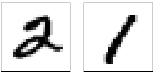
有没有更简单易懂的基准呢?让我们来尝试一个非常简单的想法:比较图片灰度。例如,一个2的图片会比1的图片黑,因为2的黑点比较多。 如下图:
建议试用训练数据来计算每个像素的平均灰度0,1,2,…,9。 当出现一个新图片,我们计算这个图片到底有多黑,然后猜测最接近哪个数字的平均灰度。这是一个简单的过程,代码也容易实现,所有我就不给出明确的代码了 - 如果你感兴趣就到GitHub去看 GitHub repository。 这是对随机猜测的改善,如果10,000次测试有2,225次正确,那么精度就为22.25%。
用上面的方法实现精度达20%到50%之间并不难。如果你努力一点可以超过50%。但是要获得更高的进度就有借助于机器学习算法了。 让我们使用一个著名的算法 support vector machine 简称 SVM算法。如果你不熟悉SVM,不用担心,我们不用了解算法的细节,我们直接用实现了Python接口的C语言类库 scikit-learn,里面提供了SVM的具体算法实现 LIBSVM。
如果你使用默认设置运行scikit-learn的 SVM 分类器,精度大概是94.35% (代码在这里 here) 比起上面的利用灰度来分类有天大的改善。事实上这里的 SVM 的性能比神经网络稍微查一点。在后面的一章我们会引进一种新的技术来改善神经网络,让它的性能比SVM出色。
然而,这不是故事的结尾。94.35%这个结果scikit-learn的SVM默认设置时的性能。 SVM有一大堆可调的参数,有可能找到一些参数来提高性能。我不会明确地去做这件事,看这里由 Andreas Mueller写的 这篇博客 如果你想了解更多。Mueller给我们演示了通过一些方法来优化SVM的参数,可以将精度提高到98.5%。换句话讲,一个好的可调的SVM出错率大0七十分之一。这非常厉害!神经网络能做得更好吗?
事实上,神经网络可以做得更好。现在,一个设计良好的神经网络处理MNIST数据方面的精度比其它算法要好,包括SVM。 当前时间 (2013年)的记录的分类的精度达到99.79%( 9,979/10,000)。这是 Li Wan, Matthew Zeiler, Sixin Zhang, Yann LeCun, 和Rob Fergus做到的。在本书的后面,我们会看到他们使用的大多数技术。这个水平的性能已经接近人类的水平了,甚至可能比人类还好一点,因为有少量的MNIST图片甚至人类都没有信心识别出来,例如:
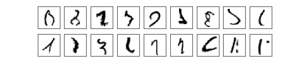
我相信你会同意上面这些图片很难区分! 上面这些MNIST图片, 21 张这样的图片放在10,000图片中神经网络能准确地识别出来。通常,编程的时候我们相信解决一个诸如识别MNIST图片数字需要一种深奥的算法。但关于我们在本章节看到算法原型,即使在Wan et al 论文中也提到神经网络仅涉及一种非常简单的算法。所有的复杂性在于神经网络从训练数据中自动学习。在某种意义上,我们实现的神经网络和其它更深奥的论文是为了解决以下问题:
向深度学习迈进
译者注:最后翻译进度的时间是:2017-01-11 00:41,我会继续往下翻译的:
我们的神经网络的性能令人印象深刻,性能有点神秘。权重和偏移会自动调整。这意味着我们不能一下子解释出神经网络是怎样做到的。我们可以找到一些方法类理解我们的神经网络怎样分类手写数字的法则吗?如果有一些法则我们会做得更好吗?
为了使这个问题更加分明,假定几十年后神经网络导致人工智能(AI)出现了。我们可以知道这种智能地神经网络是怎样工作的吗?或许网络对我们来说是透明的,权重偏移量我们不能理解,因为他们自主学习了。早些时候的AI研究,人们希望建立AI的努力可以帮助我们理解智能背后的法则和人类大脑的运行机理。最后结果可能是我们既不了解大脑的运行机制也不知道人工智能怎么工作!
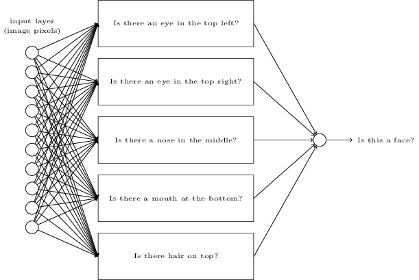
为了解决这个问题,让我们回想一下我再第一章开头提到的人工神经元的解释,衡量证据的一种手段。假如我们想判断一张图片是否是人脸:

.jpg)

我们可以用手写数字识别的相同方法类解决这个问题 - 使用图片中的像素作为神经网络的输入,一个神经元输入"是的这是一张脸" 或者 "不是,这不是脸"(这翻译有点硬)
让我们假设我们来做这件事,但我们不使用现有的学习算法。我们准备尝试手动设计一个网络,选择合适的权重和偏移量。我们应该怎么做? 先把神经网络的概念完全忘掉,我们可以将问题分解成一个个小问题:图片左上角有没有一个眼睛?右上角有没有一个眼睛?中间有鼻子吗?下边中间有没有一个嘴巴等等。
如上上面的问题的答案是 "yes",或者很可能是"yes",那么我们认为这张图片很可能是一张脸。相反,如果大多数答案都是 "no",那么图片很可能不是一张脸。
当然这只是一个粗暴的思维探索,有很多缺陷。也许这个人是光头,因此没有头发。也许我们只能看到半张脸,或者脸的某个角度,因此很多面部特征模糊不清。但这个思维探索表明如果我们用神经网络来解答这些子问题,通过这些子问题组合形成的网络,那么很可能我们可以建立一个用于脸部识别的神经网络。这是大概的架构,用矩形来代表子网络。注意这不是一个解决面部识别问题的现实中应用的方法;只是一个帮助我们建立神经网络直觉。这是架构图:
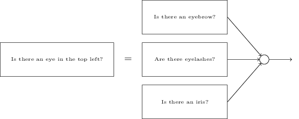
子网络貌似也可以分解。假如我们考虑一个问题:"左上角有一个眼睛吗?" 这个问题可以分解为:"是否有眼珠?"; "是否有眼睫毛?"; "是否有虹膜?";以及其它等等。当然这些问题也真的包含位置信息 - "眼珠在左上方,在睫毛的上面?", 诸如此类- 但我们为了保持简单。网络只分解一个问题, "左上方是否眼睛?" 现在可以分解成:
这些问题可以通过多层网络一步步分解。最后我们子网络可以回答到能从像素级别的回答的问题。这些问题可能,例如在图片的特定的点上的非常简单的形状。这些问题可以用一个连接到图片像素的神经元来回答。
最后的结果是一个复杂问题的网络 - (用来判断图片是否是一张脸的网络) - 分解成一个个能在单个像素级别回答的非常简单的问题。它通过分成很多层来分解问题。前几层回答图片输入的特定的简单问题,后面的层建立更复杂和抽象的概念。这种多层结构的网络 - 有两个或者更多的隐藏层 - 被叫做深度神经网络。
当然,我没有说过怎样递归分解成子网络。当然不是手工来设计权重和偏移量,我们用学习算法来搞,这样网络就可以从训练数据中自动学习调整权重和偏移量了。研究人员在1980和1990年代尝试使用随机梯度下降和反向传播算法来训练深度网络。不幸的是,除了少量特殊的架构,其它的就没有那么幸运得出心仪的结果。 网络会学习,但是太慢,在实践中没有多大作用。
2006年以来,一系列可用的深度学习神经网络的新技术被开发出来。这些深度学习技术也是基于随机梯度下降算法和反向传播算法的,但也引入了新的思想。 这些技术能够训练更深更大型的网络 - 人们现在通常能训练有5到10个隐藏层的网络,性能比原来的浅层网络(例如只有一个隐藏层的网络)要好很多。理由当然是深度网络的能力能建立复杂的概念。这有点像传统的编程语言使用模块化设计思想来抽象来构造一个复杂的程序。对比深度网络和浅层网络有点像对比有函数封装概念和没有函数概念的编程语言。当然神经网络的抽象和传统编程的抽象是不同的,只是想说明抽象真的非常重要。
译者注:至此所有浅层神经网络部分翻译都完成了,翻译完成的时间是:2017-01-22 23:35,接下来将会翻译有关深度神经网络和深度学习方面的知识,敬请期待。由于没太多时间,可能会有翻译不通顺,错别字等情况,请见谅,后面我会逐步回头检查修正,请见谅!