前言
经常用R处理数据的分析师都会对dplyr包情有独钟,它强大的数据整理功能让原始数据从杂乱无章到有序清晰,便于后期进一步的深入分析,特别是配合上数据库的使用,更是让分析师如虎添翼,轻松搞定Excel难以驾驭的数据容量,下面我们通过一个实用案例来具体看看如何将R和数据库完美融合在一起。在以后的博客中我们还会陆续讲解dplyr包的各种功能和用SQL语言访问数据库的方法。
dplyr包可以配合一系列数据库使用,如:sqlite, mysql and postgresql。这里我们着重探讨sqlite。
数据的介绍
首先我们来熟悉一下即将用到的数据,在美国,药品的检疫是个严谨的过程,当患者在服用药物后有任何不适反应,都可以将情况反映给相关部门(FDA),而这些收集来的数据也对大众公开,可以下载和分析。在这篇博客里我们会用到有关患者的人口统计信息和针对某种症状患者使用了特定药物,因为中美药物间的差别,我们暂时没有加入所用药品的信息,如果读者感兴趣,可以自行调整分析的范围,这里作者用较少数据力求让读者快速理解如何用R来读取网络数据,将其存入数据库,并融合数据集,然后做深入分析。
系统准备
library(dplyr)
library(ggplot2)
library(data.table)
library(magrittr)
下载数据
首先我们建立循环语句来下载2015上半年的季度性数据(如果空间允许,还可以建立双循环下载多于一年的数据)
year=2015
for (m in (1:2) ){
            url1<-paste0("http://www.nber.org/fda/faers/",year,"/demo",year,"q",m,".csv.zip")
                download.file(url1,dest="data.zip") # Demography
                unzip ("data.zip")
            url2<-paste0("http://www.nber.org/fda/faers/",year,"/indi",year,"q",m,".csv.zip")
                download.file(url2,dest="data.zip") # Indication
                unzip ("data.zip")
            }
解析下载数据,构建人口统计信息和反应症状数据集
filenames <- list.files(pattern="^demo.*.csv", full.names=TRUE)
demography = rbindlist(lapply(filenames, fread, select=c("primaryid","caseid","age","event_dt","sex","wt","occr_country")))
str(demography)
## Classes 'data.table' and 'data.frame':   606551 obs. of  7 variables:
##  $ primaryid   : int  35032933 36655882 38671183 38775713 38783443 40954634 41149942 41352566 41943882 42207644 ...
##  $ caseid      : int  3503293 3665588 3867118 3877571 3878344 4095463 4114994 4135256 4194388 4220764 ...
##  $ event_dt    : int  20000118 NA 20021015 NA NA 20040204 200011 200303 20040321 200404 ...
##  $ age         : num  39 35 54 NA 66 ...
##  $ sex         : chr  "F" "F" "F" "M" ...
##  $ wt          : num  83 NA 70 NA NA NA NA NA 60.8 NA ...
##  $ occr_country: chr  "US" "DE" "US" "GB" ...
##  - attr(*, ".internal.selfref")=<externalptr>

filenames <- list.files(pattern="^indi.*.csv", full.names=TRUE)
indication = rbindlist(lapply(filenames, fread, select=c("primaryid","indi_drug_seq","indi_pt")))
str(indication)
## Classes 'data.table' and 'data.frame':   1409632 obs. of  3 variables:
##  $ primaryid    : int  35032933 35032933 35032933 35032933 35032933 35032933 35032933 36655882 36655882 36655882 ...
##  $ indi_drug_seq: int  1 2 3 4 5 6 7 1 2 3 ...
##  $ indi_pt      : chr  "Multiple sclerosis" "Multiple sclerosis" "Depression" "Hypercholesterolaemia" ...
##  - attr(*, ".internal.selfref")=<externalptr>
创建数据库
这里我们没有给出路径,数据库于是会被建在之前已设好的工作文件夹中
my.db<- src_sqlite("adverse.events", create = T) # create =T creates a new database
#mysql示例
my.db<- src_mysql("####",host="#.#.#.#",port=####,user="####",password="########")
上载数据集到建好的数据库中
copy_to(my.db,demography,temporary = FALSE) # uploading demography data
## Source: sqlite 3.8.6 [adverse.events]
## From: demography [606,551 x 7]
##
##    primaryid  caseid event_dt    age   sex    wt occr_country
##        (int)   (int)    (int)  (dbl) (chr) (dbl)        (chr)
## 1   35032933 3503293 20000118 39.000     F  83.0           US
## 2   36655882 3665588       NA 35.000     F    NA           DE
## 3   38671183 3867118 20021015 54.000     F  70.0           US
## 4   38775713 3877571       NA     NA     M    NA           GB
## 5   38783443 3878344       NA 66.000     M    NA           IT
## 6   40954634 4095463 20040204 65.476     F    NA           JP
## 7   41149942 4114994   200011 17.000     F    NA
## 8   41352566 4135256   200303 46.000     F    NA           US
## 9   41943882 4194388 20040321 75.000     F  60.8
## 10  42207644 4220764   200404 18.000     F    NA           US
## ..       ...     ...
copy_to(my.db,indication,temporary = FALSE) # uploading indication data
## Source: sqlite 3.8.6 [adverse.events]
## From: indication [1,409,632 x 3]
##
##    primaryid indi_drug_seq                          indi_pt
##        (int)         (int)                            (chr)
## 1   35032933             1               Multiple sclerosis
## 2   35032933             2               Multiple sclerosis
## 3   35032933             3                       Depression
## 4   35032933             4            Hypercholesterolaemia
## 5   35032933             5 Benign neoplasm of thyroid gland
## 6   35032933             6                       Depression
## 7   35032933             7                       Depression
## 8   36655882             1         Schizoaffective disorder
## 9   36655882             2         Schizoaffective disorder
## 10  36655882             3         Schizoaffective disorder
## ..       ...           ...       ...
建立与已有数据库的链接并检索所存数据表
my.db <- src_sqlite("adverse.events", create = F) # create = F to connect to an existing databasesrc_tbls(my.db)
## [1] "demography"   "indication"   "sqlite_stat1"
访问数据库
dplyr包的命令可以借助SQL语言来对数据库中的数据进行整理,首先我们用tbl来从数据库中导入数据
demography = tbl(my.db,"demography")
head(demography)
##   primaryid  caseid event_dt    age sex wt occr_country
## 1  35032933 3503293 20000118 39.000   F 83           US
## 2  36655882 3665588       NA 35.000   F NA           DE
## 3  38671183 3867118 20021015 54.000   F 70           US
## 4  38775713 3877571       NA     NA   M NA           GB
## 5  38783443 3878344       NA 66.000   M NA           IT
## 6  40954634 4095463 20040204 65.476   F NA           JP
indication = tbl(my.db,"indication")
head(indication)
##   primaryid indi_drug_seq                          indi_pt
## 1  35032933             1               Multiple sclerosis
## 2  35032933             2               Multiple sclerosis
## 3  35032933             3                       Depression
## 4  35032933             4            Hypercholesterolaemia
## 5  35032933             5 Benign neoplasm of thyroid gland
## 6  35032933             6                       Depression
FR = filter(demography, occr_country=='FR')  # Filtering demography of patients from FranceFR$query
## <Query> SELECT "primaryid", "caseid", "event_dt", "age", "sex", "wt", "occr_country"
## FROM "demography"
## WHERE "occr_country" = 'FR'
## <SQLiteConnection>
explain(FR)
## <SQL>
## SELECT "primaryid", "caseid", "event_dt", "age", "sex", "wt", "occr_country"
## FROM "demography"
## WHERE "occr_country" = 'FR'
##
##
## <PLAN>
##   selectid order from                detail
## 1        0     0    0 SCAN TABLE demography
-
通过检索美国患者的信息可以看到dplyr包的命令自行产生的数据库检索语句
-
dplyr包的命令(
select,arrange,filter,mutate,summarize,rename)皆可用于修理数据库中的数据,我们还可以用magrittr包中的pipe功能(%>%)将多重命令链接在一起
数据分析 + 可视化ggplot
外行人经常认为数据分析师的工作不明觉厉,绘制漂亮高大上的图表,然后从纷繁的数据中探索趋势现象,但业内的人都有这样的体会,很多工作都是洗数据的“体力活”,和真正的数据分析相比,占据了分析师的大量时间和精力。比如我们在做下面几个数据分析例子前,完全可以再多花些时间将数据整理的更完善,这一块我们将会在以后的文章中详解。
demography %>%
group_by(country=occr_country) %>%
summarize(total=n()) %>% arrange(desc(total)) %>%
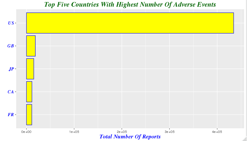
filter(country!='') %>% head(5) ## country total ## 1 US 434526 ## 2 GB 18680 ## 3 JP 15384 ## 4 CA 11530 ## 5 FR 11274
demography %>%
group_by(country=occr_country) %>%
summarize(total=n()) %>%
arrange(desc(total)) %>%
filter(country!='') %>%
head(5) %>%
mutate(country = factor(country,levels = country[order(total)])) %>%
ggplot(aes(x=country,y=total))+geom_bar(stat='identity',color='blue',fill='yellow')+xlab("")+
ggtitle('Top Five Countries With Highest Number Of Adverse Events')+theme(plot.title=element_text(size=rel(1.6),  lineheight=.9, family="Times", face="bold.italic", colour="dark green"))+coord_flip()+ylab('Total Number Of Reports')+
theme(axis.title.x=element_text(size=15, lineheight=.9, family="Times", face="bold.italic", colour="blue"))+
theme(axis.text.y=element_text(size=12,family="Times", face="bold.italic", colour="blue"))
-
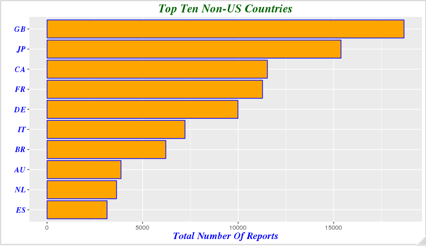
我们注意到由于美国患者人数的众多,使得其他国家的差异在横轴上不再明显,于是我们剔除美国的影响,以便观察不适反应报告较多的其他国家的差异
demography %>%
group_by(country=occr_country) %>%
summarize(total=n()) %>%
arrange(desc(total)) %>%
filter(country!='' & country!='US') %>%
head(10) %>%
mutate(country = factor(country,levels = country[order(total)])) %>%
ggplot(aes(x=country,y=total))+geom_bar(stat='identity',color='blue',fill='orange')+xlab("")+
ggtitle('Top Ten Non-US Countries')+theme(plot.title=element_text(size=rel(1.6),  lineheight=.9, family="Times", face="bold.italic", colour="dark green"))+coord_flip()+ylab('Total Number Of Reports')+
theme(axis.title.x=element_text(size=15, lineheight=.9, family="Times", face="bold.italic", colour="blue"))+
theme(axis.text.y=element_text(size=12,family="Times", face="bold.italic", colour="blue"))
indication %>%
group_by(indi_pt) %>%
summarise(count=n()) %>%
arrange(desc(count)) %>%
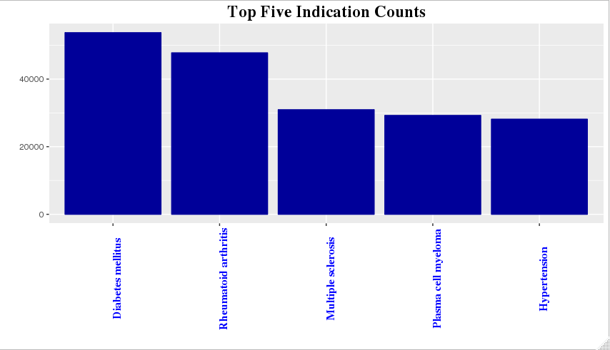
head(5) ## indi_pt count ## 1 Product used for unknown indication 463524 ## 2 Diabetes mellitus 53742 ## 3 Rheumatoid arthritis 47780 ## 4 Multiple sclerosis 30946 ## 5 Plasma cell myeloma 29256
indication %>%
group_by(indi_pt) %>%
summarise(count=n()) %>%
arrange(desc(count)) %>%
head(6) %>%
tail(-1) %>%
mutate(indi_pt=factor(indi_pt,levels = indi_pt[order(desc(count))])) %>%
ggplot(aes(x=indi_pt, y=count))+
  geom_bar(stat='identity',colour="#000099",fill="#000099")+ggtitle('Top Five Indication Counts') + xlab('') +
  ylab('')+theme(plot.title =element_text(size = rel(1.6), family="Times", face="bold", colour = "black"))+
  theme(axis.text.x=element_text(angle=90, size=12,family="Times", face="bold", colour="blue"))
-
我们剔除了计数最多的一项,即不明确患者症状
-
图表表明针对肥胖的药物记录了最多的不适症状,在美国这一现象比较符合预期,众所周知的人口肥胖问题使相关药物使用较为普遍
年龄的分布
-
基本分布函数
hist,qplot,和ggplot都能用于作图 -
在这里我们移除了小于0和大于100的年龄记录,这种不符合现实情况的异常值可能源于数据录入出错等原因
demography$age <- round(as.numeric(demography$age))
demography %>%
filter(!is.na(age) & age<100 & age>0) %>%
select(age) %>%
as.data.frame() %>%
ggplot(aes(x=age))+
  geom_histogram(breaks=seq(0, 100, by =5), col="dark grey", aes(fill=..count..)) +
  scale_fill_gradient("Count", low = "green", high = "red")+labs(title="Age Histogram") +labs(x="Age",y="")+
  theme(plot.title =element_text(size = rel(1.6), family="Times", face="bold", colour = "black"))+
  theme(axis.text.x=element_text(size=10,family="Times", face="bold", colour="black"))+
  theme(axis.title.x=element_text(size=12,family="Times", face="bold", colour="black"))

合并数据集
joined = demography %>%
inner_join(indication, by='primaryid',copy = TRUE) head(joined,5)
##   primaryid  caseid event_dt age sex wt occr_country indi_drug_seq
## 1  35032933 3503293 20000118  39   F 83           US             1
## 2  35032933 3503293 20000118  39   F 83           US             2
## 3  35032933 3503293 20000118  39   F 83           US             3
## 4  35032933 3503293 20000118  39   F 83           US             4
## 5  35032933 3503293 20000118  39   F 83           US             5
##                            indi_pt
## 1               Multiple sclerosis
## 2               Multiple sclerosis
## 3                       Depression
## 4            Hypercholesterolaemia
## 5 Benign neoplasm of thyroid gland
-
关于合并数据集的操作有很多种,作者在这里展示了比较常用的inner_join,而还有right_join,left_join,full_join,semi_join,anti_join等等的操作可供选择,我们会在以后的文章中具体探讨。