Building Particle Filters and Particle MCMC in NIMBLE

This example shows how to construct and conduct inference on a state space model using particle filtering algorithms. nimblecurrently has versions of the bootstrap filter, the auxiliary particle filter, the ensemble Kalman filter, and the Liu and West filter implemented. Additionally, particle MCMC samplers are available and can be specified for both univariate and multivariate parameters.

Model Creation

## load the nimble library and set seed
library('nimble')
set.seed(1)

## define the model
stateSpaceCode <- nimbleCode({
    a ~ dunif(-0.9999, 0.9999)
    b ~ dnorm(0, sd = 1000)
    sigPN ~ dunif(1e-04, 1)
    sigOE ~ dunif(1e-04, 1)
    x[1] ~ dnorm(b/(1 - a), sd = sigPN/sqrt((1-a*a)))
    y[1] ~ dt(mu = x[1], sigma = sigOE, df = 5)
    for (i in 2:t) {
        x[i] ~ dnorm(a * x[i - 1] + b, sd = sigPN)
        y[i] ~ dt(mu = x[i], sigma = sigOE, df = 5)
    }
})

## define data, constants, and initial values  
data <- list(
    y = c(0.213, 1.025, 0.314, 0.521, 0.895, 1.74, 0.078, 0.474, 0.656, 0.802)
)
constants <- list(
    t = 10
)
inits <- list(
    a = 0,
    b = .5,
    sigPN = .1,
    sigOE = .05
)

## build the model
stateSpaceModel <- nimbleModel(stateSpaceCode,
                              data = data,
                              constants = constants,
                              inits = inits,
                              check = FALSE)

## defining model...

## building model...

## setting data and initial values...

## running calculate on model (any error reports that follow may simply
## reflect missing values in model variables) ...

## 

## checking model sizes and dimensions...

## note that missing values (NAs) or non-finite values were found in model
## variables: x, lifted_a_times_x_oBi_minus_1_cB_plus_b. This is not an error,
## but some or all variables may need to be initialized for certain algorithms
## to operate properly.

## 

## model building finished.

Construct and run a bootstrap filter

We next construct a bootstrap filter to conduct inference on the latent states of our state space model. Note that the bootstrap filter, along with the auxiliary particle filter and the ensemble Kalman filter, treat the top-level parameters a, b, sigPN, and sigOEas fixed. Therefore, the bootstrap filter below will proceed as though a = 0, b = .5, sigPN = .1, and sigOE = .05, which are the initial values that were assigned to the top-level parameters.

The bootstrap filter takes as arguments the name of the model and the name of the latent state variable within the model. The filter can also take a control list that can be used to fine-tune the algorithm’s configuration.

## build bootstrap filter and compile model and filter
bootstrapFilter <- buildBootstrapFilter(stateSpaceModel, nodes = 'x')
compiledList <- compileNimble(stateSpaceModel, bootstrapFilter)

## compiling... this may take a minute. Use 'showCompilerOutput = TRUE' to see C++ compiler details.

## compilation finished.

## run compiled filter with 10,000 particles.  
## note that the bootstrap filter returns an estimate of the log-likelihood of the model.
compiledList$bootstrapFilter$run(10000)

## [1] -28.13009

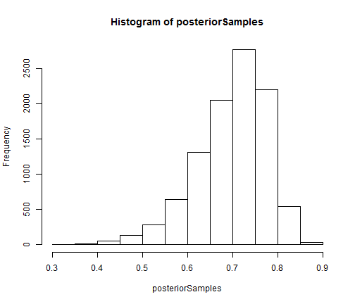
Particle filtering algorithms in nimble store weighted samples of the filtering distribution of the latent states in the mvSamplesmodelValues object. Equally weighted samples are stored in the mvEWSamples object. By default, nimble only stores samples from the final time point.

## extract equally weighted posterior samples of x[10]  and create a histogram
posteriorSamples <- as.matrix(compiledList$bootstrapFilter$mvEWSamples)
hist(posteriorSamples)

The auxiliary particle filter and ensemble Kalman filter can be constructed and run in the same manner as the bootstrap filter.

Conduct inference on top-level parameters using particle MCMC

Particle MCMC can be used to conduct inference on the posterior distribution of both the latent states and any top-level parameters of interest in a state space model. The particle marginal Metropolis-Hastings sampler can be specified to jointly sample the a, b, sigPN, and sigOE top level parameters within nimble‘s MCMC framework as follows:

## create MCMC specification for the state space model
stateSpaceMCMCconf <- configureMCMC(stateSpaceModel, nodes = NULL)

## add a block pMCMC sampler for a, b, sigPN, and sigOE 
stateSpaceMCMCconf$addSampler(target = c('a', 'b', 'sigPN', 'sigOE'),
                              type = 'RW_PF_block', control = list(latents = 'x'))

## build and compile pMCMC sampler
stateSpaceMCMC <- buildMCMC(stateSpaceMCMCconf)
compiledList <- compileNimble(stateSpaceModel, stateSpaceMCMC, resetFunctions = TRUE)

## compiling... this may take a minute. Use 'showCompilerOutput = TRUE' to see C++ compiler details.

## compilation finished.

## run compiled sampler for 5000 iterations
compiledList$stateSpaceMCMC$run(5000)

## |-------------|-------------|-------------|-------------|
## |-------------------------------------------------------|

## NULL

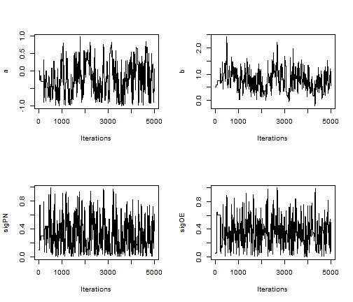
## create trace plots for each parameter
library('coda')

par(mfrow = c(2,2))
posteriorSamps <- as.mcmc(as.matrix(compiledList$stateSpaceMCMC$mvSamples))
traceplot(posteriorSamps[,'a'], ylab = 'a')
traceplot(posteriorSamps[,'b'], ylab = 'b')
traceplot(posteriorSamps[,'sigPN'], ylab = 'sigPN')
traceplot(posteriorSamps[,'sigOE'], ylab = 'sigOE')

The above RW_PF_block sampler uses a multivariate normal proposal distribution to sample vectors of top-level parameters. To sample a scalar top-level parameter, use the RW_PF sampler instead.

转自：https://r-nimble.org/building-particle-filters-and-particle-mcmc-in-nimble-2