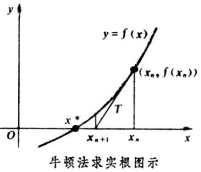
1. 牛顿法求方程的根
假设我们需求$f(x)=0$的根,并假设$f(x)=0$可导。首先,把$f(x)$在$x_0$进行一阶泰勒展开:
![]()
由$f(x)=0$可得:
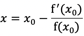
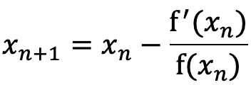
因此迭代公式为:
2. 牛顿法求极小值

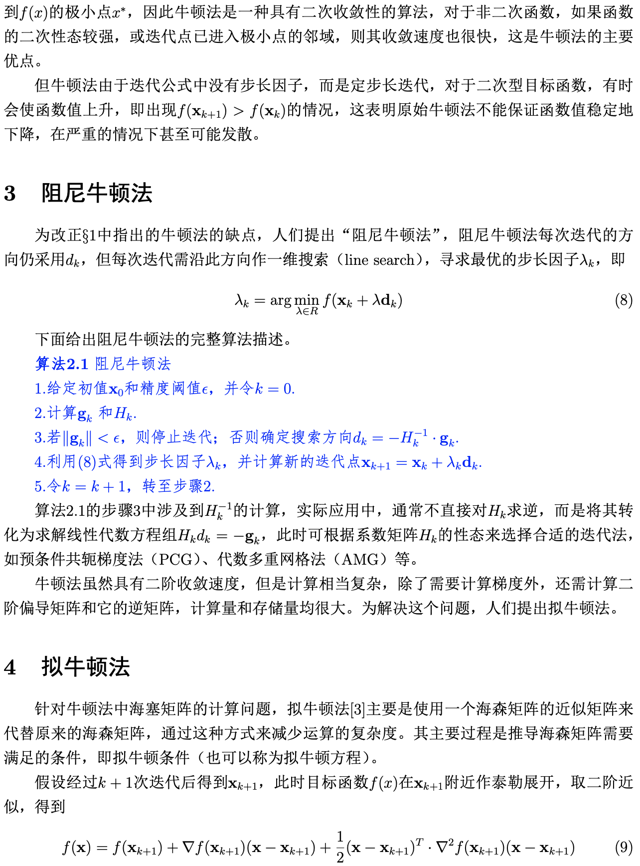


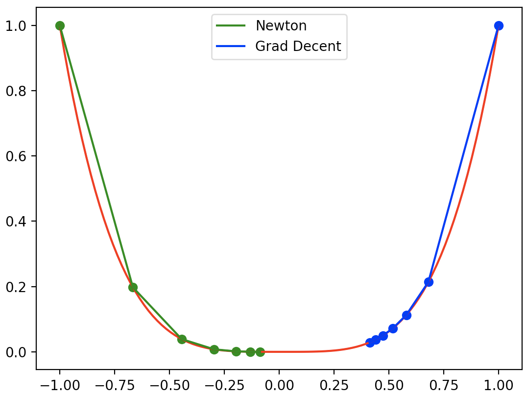
6. 牛顿法和梯度下降法的比较
这里我们用一个简单的例子比较牛顿法和梯度下降法的收敛效果:求$f(x)=x^4$的极小值。实现代码如下:
import numpy as np
import matplotlib.pyplot as plt


# 目标函数:y=x^4
def func(x):
    return x**4


# 目标函数一阶导数:dy/dx=2*x
def dfunc(x):
    return 4 * x**3


# 目标函数二阶导数
def ddfunc(x):
    return 12 * x**2


# Newton method
def newton(x_start, epochs):
    """
    牛顿迭代法。给定起始点与目标函数的一阶导函数和二阶导数,求在epochs次迭代中x的更新值
    :param x_start: x的起始点
    :param epochs: 迭代周期
    :return: x在每次迭代后的位置(包括起始点),长度为epochs+1
    """
    xs = np.zeros(epochs+1)
    x = x_start
    xs[0] = x
    for i in range(epochs):
        delta_x = -(dfunc(x)/ddfunc(x))
        x += delta_x
        xs[i+1] = x
    return xs


# Gradient Descent
def GD(x_start, epochs, lr):
    """
    梯度下降法。给定起始点与目标函数的一阶导函数,求在epochs次迭代中x的更新值
    :param x_start: x的起始点
    :param epochs: 迭代周期
    :param lr: 学习率
    :return: x在每次迭代后的位置(包括起始点),长度为epochs+1
    """
    xs = np.zeros(epochs+1)
    x = x_start
    xs[0] = x
    for i in range(epochs):
        dx = dfunc(x)
        # v表示x要改变的幅度
        v = - dx * lr
        x += v
        xs[i+1] = x
    return xs


line_x = np.linspace(-1, 1, 100)
line_y = func(line_x)

x_start_newton = -1
x_start_GD = 1
epochs = 6

lr = 0.08
x_newton = newton(x_start_newton, epochs)
x_GD = GD(x_start_GD, epochs, lr=lr)

plt.plot(line_x, line_y, c='r')

color_newton = 'g'
plt.plot(x_newton, func(x_newton), c=color_newton, label='Newton')
plt.scatter(x_newton, func(x_newton), c=color_newton, )

color_GD = 'b'
plt.plot(x_GD, func(x_GD), c=color_GD, label='Grad Decent')
plt.scatter(x_GD, func(x_GD), c=color_GD, )

plt.legend()
plt.show()
结果如下,梯度下降算法的收敛效果受学习率影响: