本文主要包括:
- 一、什么是LSTM
- 二、LSTM的曲线拟合
- 三、LSTM的分类问题
- 四、为什么LSTM有助于消除梯度消失
一、什么是LSTM
Long Short Term 网络即为LSTM,是一种循环神经网络(RNN),可以学习长期依赖问题。RNN 都具有一种重复神经网络模块的链式的形式。在标准的 RNN 中,这个重复的模块只有一个非常简单的结构,例如一个 tanh 层。
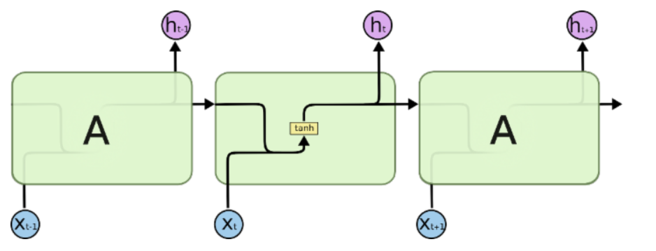
如上为标准的RNN神经网络结构,LSTM则与此不同,其网络结构如图:
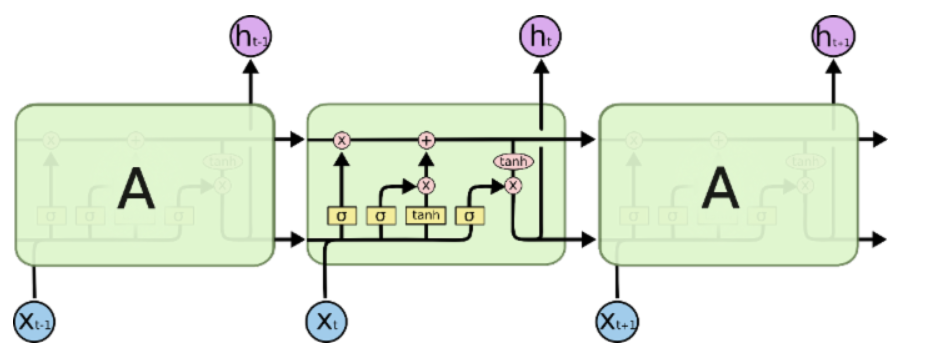
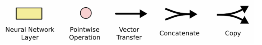
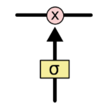
其中,网络中各个元素图标为:
LSTM 通过精心设计的称作为“门”的结构来去除或者增加信息到细胞状态的能力。门是一种让信息选择式通过的方法。他们包含一个 sigmoid 神经网络层和一个 pointwise 乘法操作。LSTM 拥有三个门,来保护和控制细胞状态。
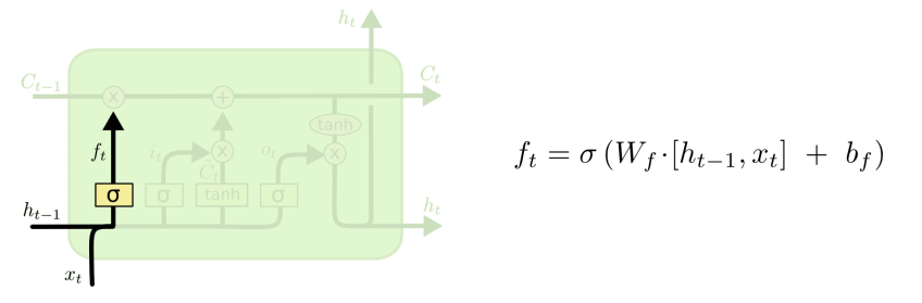
首先是忘记门:
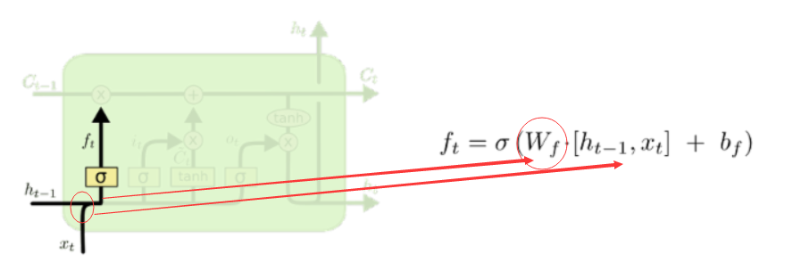
如上,忘记门中需要注意的是,训练的是一个wf的权值,而且上一时刻的输出和当前时刻的输入是一个concat操作。忘记门决定我们会从细胞状态中丢弃什么信息,因为sigmoid函数的输出是一个小于1的值,相当于对每个维度上的值做一个衰减。
然后是信息增加门,决定了什么新的信息到细胞状态中:
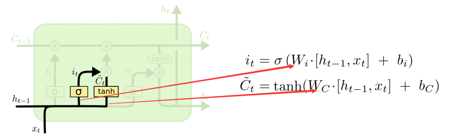
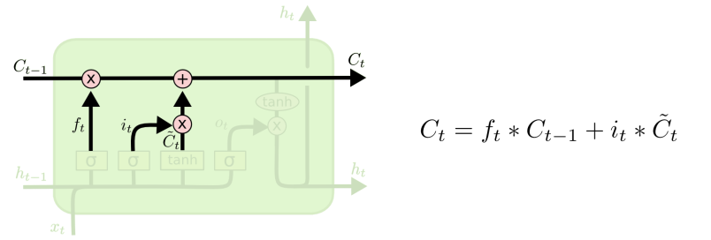
其中,sigmoid决定了什么值需要更新,tanh创建一个新的细胞状态的候选向量Ct,该过程训练两个权值Wi和Wc。经过第一个和第二个门后,可以确定传递信息的删除和增加,即可以进行“细胞状态”的更新。
第三个门就是信息输出门:
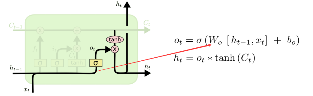
通过sigmoid确定细胞状态那个部分将输出,tanh处理细胞状态得到一个-1到1之间的值,再将它和sigmoid门的输出相乘,输出程序确定输出的部分。
二、LSTM的曲线拟合
2.1 股票价格预测
下面介绍一个网上常用的利用LSTM做股票价格的回归例子,数据:
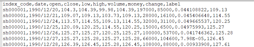
如上,可以看到用例包含:index_code,date,open,close,low,high,volume,money,change这样几个特征。提取特征从open-change个特征,作为神经网络的输入,输出即为label。整个代码如下:
import pandas as pd
import numpy as np
import matplotlib.pyplot as plt
import tensorflow as tf
#定义常量
rnn_unit=10 #hidden layer units
input_size=7
output_size=1
lr=0.0006 #学习率
#——————————————————导入数据——————————————————————
f=open('dataset_2.csv')
df=pd.read_csv(f) #读入股票数据
data=df.iloc[:,2:10].values #取第3-10列
#获取训练集
def get_train_data(batch_size=60,time_step=20,train_begin=0,train_end=5800):
batch_index=[]
data_train=data[train_begin:train_end]
normalized_train_data=(data_train-np.mean(data_train,axis=0))/np.std(data_train,axis=0) #标准化
train_x,train_y=[],[] #训练集
for i in range(len(normalized_train_data)-time_step):
if i % batch_size==0:
batch_index.append(i)
x=normalized_train_data[i:i+time_step,:7]
y=normalized_train_data[i:i+time_step,7,np.newaxis]
train_x.append(x.tolist())
train_y.append(y.tolist())
batch_index.append((len(normalized_train_data)-time_step))
return batch_index,train_x,train_y
#获取测试集
def get_test_data(time_step=20,test_begin=5800):
data_test=data[test_begin:]
mean=np.mean(data_test,axis=0)
std=np.std(data_test,axis=0)
normalized_test_data=(data_test-mean)/std #标准化
size=(len(normalized_test_data)+time_step-1)//time_step #有size个sample
test_x,test_y=[],[]
for i in range(size-1):
x=normalized_test_data[i*time_step:(i+1)*time_step,:7]
y=normalized_test_data[i*time_step:(i+1)*time_step,7]
test_x.append(x.tolist())
test_y.extend(y)
test_x.append((normalized_test_data[(i+1)*time_step:,:7]).tolist())
test_y.extend((normalized_test_data[(i+1)*time_step:,7]).tolist())
return mean,std,test_x,test_y
#——————————————————定义神经网络变量——————————————————
#输入层、输出层权重、偏置
weights={
'in':tf.Variable(tf.random_normal([input_size,rnn_unit])),
'out':tf.Variable(tf.random_normal([rnn_unit,1]))
}
biases={
'in':tf.Variable(tf.constant(0.1,shape=[rnn_unit,])),
'out':tf.Variable(tf.constant(0.1,shape=[1,]))
}
#——————————————————定义神经网络变量——————————————————
def lstm(X):
batch_size=tf.shape(X)[0]
time_step=tf.shape(X)[1]
w_in=weights['in']
b_in=biases['in']
input=tf.reshape(X,[-1,input_size]) #需要将tensor转成2维进行计算,计算后的结果作为隐藏层的输入
input_rnn=tf.matmul(input,w_in)+b_in
input_rnn=tf.reshape(input_rnn,[-1,time_step,rnn_unit]) #将tensor转成3维,作为lstm cell的输入
cell=tf.nn.rnn_cell.BasicLSTMCell(rnn_unit)
init_state=cell.zero_state(batch_size,dtype=tf.float32)
output_rnn,final_states=tf.nn.dynamic_rnn(cell, input_rnn,initial_state=init_state, dtype=tf.float32) #output_rnn是记录lstm每个输出节点的结果,final_states是最后一个cell的结果
output=tf.reshape(output_rnn,[-1,rnn_unit]) #作为输出层的输入
w_out=weights['out']
b_out=biases['out']
pred=tf.matmul(output,w_out)+b_out
return pred,final_states
#——————————————————训练模型——————————————————
def train_lstm(batch_size=80,time_step=15,train_begin=2000,train_end=5800):
X=tf.placeholder(tf.float32, shape=[None,time_step,input_size])
Y=tf.placeholder(tf.float32, shape=[None,time_step,output_size])
# 训练样本中第2001 - 5785个样本,每次取15个
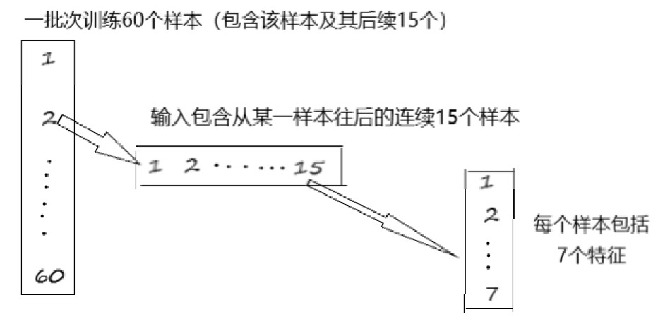
batch_index,train_x,train_y=get_train_data(batch_size,time_step,train_begin,train_end)
print(np.array(train_x).shape)# 3785 15 7
print(batch_index)
#相当于总共3785句话,每句话15个字,每个字7个特征(embadding),对于这些样本每次训练80句话
pred,_=lstm(X)
#损失函数
loss=tf.reduce_mean(tf.square(tf.reshape(pred,[-1])-tf.reshape(Y, [-1])))
train_op=tf.train.AdamOptimizer(lr).minimize(loss)
saver=tf.train.Saver(tf.global_variables(),max_to_keep=15)
with tf.Session() as sess:
sess.run(tf.global_variables_initializer())
#重复训练200次
for i in range(200):
#每次进行训练的时候,每个batch训练batch_size个样本
for step in range(len(batch_index)-1):
_,loss_=sess.run([train_op,loss],feed_dict={X:train_x[batch_index[step]:batch_index[step+1]],Y:train_y[batch_index[step]:batch_index[step+1]]})
print(i,loss_)
if i % 200==0:
print("保存模型:",saver.save(sess,'model/stock2.model',global_step=i))
train_lstm()
#————————————————预测模型————————————————————
def prediction(time_step=20):
X=tf.placeholder(tf.float32, shape=[None,time_step,input_size])
mean,std,test_x,test_y=get_test_data(time_step)
pred,_=lstm(X)
saver=tf.train.Saver(tf.global_variables())
with tf.Session() as sess:
#参数恢复
module_file = tf.train.latest_checkpoint('model')
saver.restore(sess, module_file)
test_predict=[]
for step in range(len(test_x)-1):
prob=sess.run(pred,feed_dict={X:[test_x[step]]})
predict=prob.reshape((-1))
test_predict.extend(predict)
test_y=np.array(test_y)*std[7]+mean[7]
test_predict=np.array(test_predict)*std[7]+mean[7]
acc=np.average(np.abs(test_predict-test_y[:len(test_predict)])/test_y[:len(test_predict)]) #偏差
#以折线图表示结果
plt.figure()
plt.plot(list(range(len(test_predict))), test_predict, color='b')
plt.plot(list(range(len(test_y))), test_y, color='r')
plt.show()
prediction()
这个过程并不难理解,下面分析其中维度变换,从而增加对LSTM的理解。
对于RNN的网络的构建,可以从输入张量的维度上理解,这里我们使用dynamic_rnn(当然可以注意与tf.contrib.rnn.static_rnn在使用上的区别):
dynamic_rnn(
    cell,
    inputs,
    sequence_length=None,
    initial_state=None,
    dtype=None,
    parallel_iterations=None,
    swap_memory=False,
    time_major=False,
    scope=None
)
其中:
cell:输入一个RNNcell实例
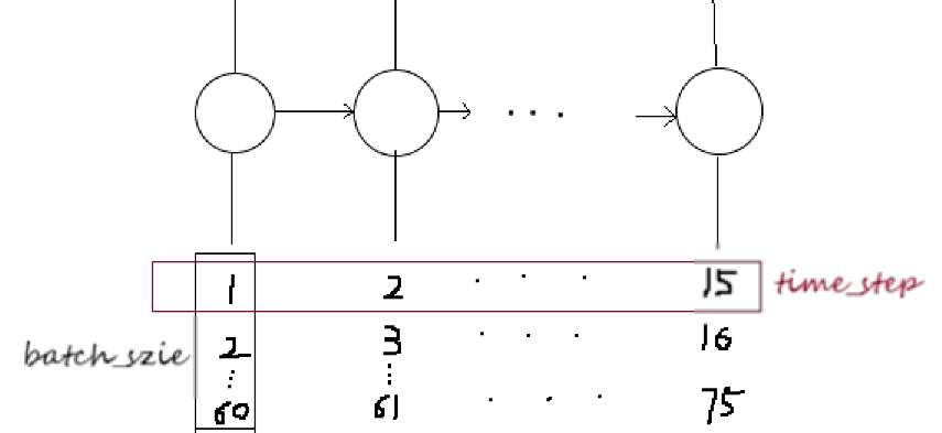
inputs:RNN神经网络的输入,如果 time_major == False (default),输入的形状是: [batch_size, max_time, embedding_size];如果 time_major == True, 输入的形状是: [ max_time, batch_size, embedding_size]
initial_state: RNN网络的初始状态,网络需要一个初始状态,对于普通的RNN网络,初始状态的形状是:[batch_size, cell.state_size]
2.2 正弦曲线拟合
对于使用LSTM做曲线拟合,参考https://morvanzhou.github.io/tutorials/machine-learning/tensorflow/5-09-RNN3/,得到代码:
import tensorflow as tf
import numpy as np
import matplotlib.pyplot as plt

BATCH_START = 0 #建立 batch data 时候的 index
TIME_STEPS = 20 # backpropagation through time 的time_steps
BATCH_SIZE = 50
INPUT_SIZE = 1 # x数据输入size
OUTPUT_SIZE = 1 # cos数据输出 size
CELL_SIZE = 10 # RNN的 hidden unit size
LR = 0.006  # learning rate

# 定义一个生成数据的 get_batch function:
def get_batch():
    #global BATCH_START, TIME_STEPS
    # xs shape (50batch, 20steps)
    xs = np.arange(BATCH_START, BATCH_START+TIME_STEPS*BATCH_SIZE).reshape((BATCH_SIZE, TIME_STEPS)) / (10*np.pi)
    res = np.cos(xs)
    # returned  xs and res: shape (batch, step, input)
    return [xs[:, :, np.newaxis], res[:, :, np.newaxis]]

# 定义 LSTMRNN 的主体结构
class LSTMRNN(object):
    def __init__(self, n_steps, input_size, output_size, cell_size, batch_size):
        self.n_steps = n_steps
        self.input_size = input_size
        self.output_size = output_size
        self.cell_size = cell_size
        self.batch_size = batch_size
        with tf.name_scope('inputs'):
            self.xs = tf.placeholder(tf.float32, [None, n_steps, input_size], name='xs')
            self.ys = tf.placeholder(tf.float32, [None, n_steps, output_size], name='ys')
        with tf.variable_scope('in_hidden'):
            self.add_input_layer()
        with tf.variable_scope('LSTM_cell'):
            self.add_cell()
        with tf.variable_scope('out_hidden'):
            self.add_output_layer()
        with tf.name_scope('cost'):
            self.compute_cost()
        with tf.name_scope('train'):
            self.train_op = tf.train.AdamOptimizer(LR).minimize(self.cost)

    # 设置 add_input_layer 功能, 添加 input_layer:
    def add_input_layer(self, ):
        l_in_x = tf.reshape(self.xs, [-1, self.input_size], name='2_2D')  # (batch*n_step, in_size)
        # Ws (in_size, cell_size)
        Ws_in = self._weight_variable([self.input_size, self.cell_size])
        # bs (cell_size, )
        bs_in = self._bias_variable([self.cell_size, ])
        # l_in_y = (batch * n_steps, cell_size)
        with tf.name_scope('Wx_plus_b'):
            l_in_y = tf.matmul(l_in_x, Ws_in) + bs_in
        # reshape l_in_y ==> (batch, n_steps, cell_size)
        self.l_in_y = tf.reshape(l_in_y, [-1, self.n_steps, self.cell_size], name='2_3D')

    # 设置 add_cell 功能, 添加 cell, 注意这里的 self.cell_init_state,
    #  因为我们在 training 的时候, 这个地方要特别说明.
    def add_cell(self):
        lstm_cell = tf.contrib.rnn.BasicLSTMCell(self.cell_size, forget_bias=1.0, state_is_tuple=True)
        with tf.name_scope('initial_state'):
            self.cell_init_state = lstm_cell.zero_state(self.batch_size, dtype=tf.float32)
        self.cell_outputs, self.cell_final_state = tf.nn.dynamic_rnn(lstm_cell,
                                                                     self.l_in_y,
                                                                     initial_state=self.cell_init_state,
                                                                     time_major=False)

    # 设置 add_output_layer 功能, 添加 output_layer:
    def add_output_layer(self):
        # shape = (batch * steps, cell_size)
        l_out_x = tf.reshape(self.cell_outputs, [-1, self.cell_size], name='2_2D')
        Ws_out = self._weight_variable([self.cell_size, self.output_size])
        bs_out = self._bias_variable([self.output_size, ])
        # shape = (batch * steps, output_size)
        with tf.name_scope('Wx_plus_b'):
            self.pred = tf.matmul(l_out_x, Ws_out) + bs_out

    # 添加 RNN 中剩下的部分:
    def compute_cost(self):
        losses = tf.contrib.legacy_seq2seq.sequence_loss_by_example(
            [tf.reshape(self.pred, [-1], name='reshape_pred')],
            [tf.reshape(self.ys, [-1], name='reshape_target')],
            [tf.ones([self.batch_size * self.n_steps], dtype=tf.float32)],
            average_across_timesteps=True,
            softmax_loss_function=self.ms_error,
            name='losses'
        )
        with tf.name_scope('average_cost'):
            self.cost = tf.div(
                tf.reduce_sum(losses, name='losses_sum'),
                self.batch_size,
                name='average_cost')
            tf.summary.scalar('cost', self.cost)

    def ms_error(self,labels, logits):
        return tf.square(tf.subtract(labels, logits))

    def _weight_variable(self, shape, name='weights'):
        initializer = tf.random_normal_initializer(mean=0., stddev=1., )
        return tf.get_variable(shape=shape, initializer=initializer, name=name)

    def _bias_variable(self, shape, name='biases'):
        initializer = tf.constant_initializer(0.1)
        return tf.get_variable(name=name, shape=shape, initializer=initializer)


# 训练 LSTMRNN
if __name__ == '__main__':

    # 搭建 LSTMRNN 模型
    model = LSTMRNN(TIME_STEPS, INPUT_SIZE, OUTPUT_SIZE, CELL_SIZE, BATCH_SIZE)
    sess = tf.Session()
    saver=tf.train.Saver(max_to_keep=3)
    sess.run(tf.global_variables_initializer())
    t = 0
    if(t == 1):
        model_file=tf.train.latest_checkpoint('model/')
        saver.restore(sess,model_file )
        xs, res = get_batch()  # 提取 batch data
        feed_dict = {model.xs: xs}
        pred = sess.run( model.pred,feed_dict=feed_dict)
        xs.shape = (-1,1)
        res.shape = (-1, 1)
        pred.shape = (-1, 1)
        print(xs.shape,res.shape,pred.shape)
        plt.figure()
        plt.plot(xs,res,'-r')
        plt.plot(xs,pred,'--g')
        plt.show()
    else:
        # matplotlib可视化
        plt.ion()  # 设置连续 plot
        plt.show()
        # 训练多次
        for i in range(2500):
            xs, res = get_batch()  # 提取 batch data
            # 初始化 data
            feed_dict = {
                model.xs: xs,
                model.ys: res,
            }
            # 训练
            _, cost, state, pred = sess.run(
                [model.train_op, model.cost, model.cell_final_state, model.pred],
                feed_dict=feed_dict)

            # plotting
            x = xs.reshape(-1,1)
            r = res.reshape(-1, 1)
            p = pred.reshape(-1, 1)
            plt.clf()
            plt.plot(x, r, 'r', x, p, 'b--')
            plt.ylim((-1.2, 1.2))
            plt.draw()
            plt.pause(0.3)  # 每 0.3 s 刷新一次

            # 打印 cost 结果
            if i % 20 == 0:
                saver.save(sess, "model/lstem_text.ckpt",global_step=i)#
                print('cost: ', round(cost, 4))
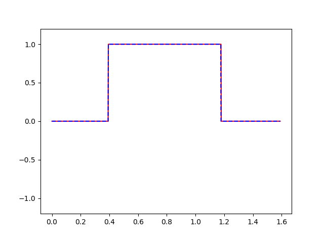
可以看到一个有意思的现象,下面是先后两个时刻的图像:

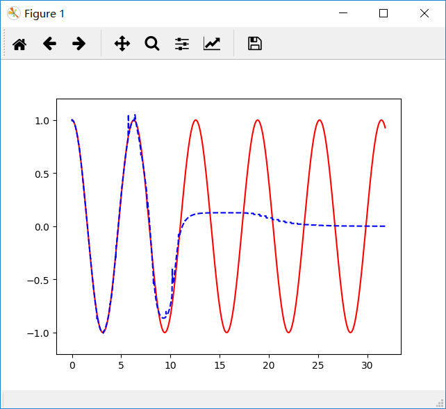
x值较小的点先收敛,x值大的收敛速度很慢。其原因主要是BPTT的求导过程,对于时间靠前的梯度下降快,可以参考:https://www.cnblogs.com/pinking/p/9418280.html 中1.2节。将网络结构改为双向循环神经网络:
def add_cell(self):
        lstm_cell = tf.contrib.rnn.BasicLSTMCell(self.cell_size, forget_bias=1.0, state_is_tuple=True)
        lstm_cell = tf.contrib.rnn.MultiRNNCell([lstm_cell],1)
        with tf.name_scope('initial_state'):
            self.cell_init_state = lstm_cell.zero_state(self.batch_size, dtype=tf.float32)
        self.cell_outputs, self.cell_final_state = tf.nn.dynamic_rnn(lstm_cell,
                                                                     self.l_in_y,
                                                                     initial_state=self.cell_init_state,
                                                                     time_major=False)
发现收敛速度快了一些。不过这个问题主要还是是因为x的值过大导致的,修改代码,将原始的值的获取进行分段:
BATCH_START = 3000 #建立 batch data 时候的 index
TIME_STEPS = 20 # backpropagation through time 的time_steps
BATCH_SIZE_r = 50
BATCH_SIZE = 10
INPUT_SIZE = 1 # x数据输入size
OUTPUT_SIZE = 1 # cos数据输出 size
CELL_SIZE = 10 # RNN的 hidden unit size
LR = 0.006  # learning rate
ii = 0
# 定义一个生成数据的 get_batch function:
def get_batch():
    global ii
    # xs shape (50batch, 20steps)
    xs_r = np.arange(BATCH_START, BATCH_START+TIME_STEPS*BATCH_SIZE_r)
    xs = xs_r[ii*BATCH_SIZE*TIME_STEPS:(ii+1)*BATCH_SIZE*TIME_STEPS].reshape((BATCH_SIZE, TIME_STEPS)) / (10*np.pi)
    res = np.cos(xs)
    ii += 1
    if(ii == 5):
        ii = 0

    # returned  xs and res: shape (batch, step, input)
    return [xs[:, :, np.newaxis], res[:, :, np.newaxis]]
然后可以具体观测某一段的收敛过程:
# matplotlib可视化
        plt.ion()  # 设置连续 plot
        plt.show()
        # 训练多次
        for i in range(200):
            xs,res,pred = [],[],[]
            for j in range(5):


                xsj, resj = get_batch()  # 提取 batch data
                if(j != 0):
                    continue
                # 初始化 data
                feed_dict = {
                    model.xs: xsj,
                    model.ys: resj,
                }
                # 训练
                _, cost, state, predj = sess.run(
                    [model.train_op, model.cost, model.cell_final_state, model.pred],
                    feed_dict=feed_dict)

            # plotting
                x = list(xsj.reshape(-1,1))
                r = list(resj.reshape(-1, 1))
                p = list(predj.reshape(-1, 1))
                xs += x
                res += r
                pred += p
            plt.clf()
            plt.plot(xs, res, 'r', x, p, 'b--')
            plt.ylim((-1.2, 1.2))
            plt.draw()
            plt.pause(0.3)  # 每 0.3 s 刷新一次

            # 打印 cost 结果
            if i % 20 == 0:
                saver.save(sess, "model/lstem_text.ckpt",global_step=i)#
                print('cost: ', round(cost, 4))
可以看到,当设置的区间比较大,譬如BATCH_START = 3000了,那么就很难收敛了。

因此,这里需要注意了,LSTM做回归问题的时候,注意观测值与自变量之间不要差距过大。当我们改小一些x的值,可以看到效果如图:
三、LSTM的分类问题
对于分类问题,其实和回归是一样的,假设在上面的正弦函数的基础上,若y大于0标记为1,y小于0标记为0,则输出变成了一个n_class(n个类别)的向量,本例中两个维度分别代表标记为0的概率和标记为1的概率。需要修改的地方为:
首先是数据产生函数,添加一个打标签的过程:
# 定义一个生成数据的 get_batch function:
def get_batch():
    #global BATCH_START, TIME_STEPS
    # xs shape (50batch, 20steps)
    xs = np.arange(BATCH_START, BATCH_START+TIME_STEPS*BATCH_SIZE).reshape((BATCH_SIZE, TIME_STEPS)) / (200*np.pi)
    res = np.where(np.cos(4*xs)>=0,0,1).tolist()
    for i in range(BATCH_SIZE):
        for j in range(TIME_STEPS):
            res[i][j] = [0,1] if res[i][j] == 1 else [1,0]
    # returned  xs and res: shape (batch, step, input/output)
    return [xs[:, :, np.newaxis], np.array(res)]
然后修改损失函数,回归问题就不能用最小二乘的损失了,可以采用交叉熵损失函数:
def compute_cost(self):
        self.cost = tf.reduce_mean(tf.nn.softmax_cross_entropy_with_logits(labels = self.ys,logits = self.pred))
当然,注意一下维度问题就可以了,效果如图:

例子代码 。
四、为什么LSTM有助于消除梯度消失
为了解决RNN的梯度问题,首先有人提出了渗透单元的办法,即在时间轴上增加跳跃连接,后推广成LSTM。LSTM其门结构,提供了一种对梯度的选择的作用。
对于门结构,其实如果关闭,则会一直保存以前的信息,其实也就是缩短了链式求导。
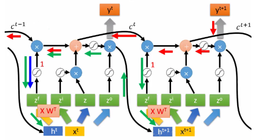
譬如,对某些输入张量训练得到的ft一直为1,则Ct-1的信息可以一直保存,直到有输入x得到的ft为0,则和前面的信息就没有关系了。故解决了长时间的依赖问题。因为门控机制的存在,我们通过控制门的打开、关闭等操作,让梯度计算沿着梯度乘积接近1的部分创建路径。

如上,可以通过门的控制,看到红色和蓝色箭头代表的路径下,yt+1的在这个路径下的梯度与上一时刻梯度保持不变。
对于信息增加门与忘记门的“+”操作,其求导是加法操作而不是乘法操作,该环节梯度为1,不会产生链式求导。如后面的求导,绿色路径和蓝色路径是相加的关系,保留了之前的梯度。

然而,梯度消失现象可以改善,但是梯度爆炸还是可能会出现的。譬如对于绿色路径:
还是存在着w导致的梯度爆炸现象。