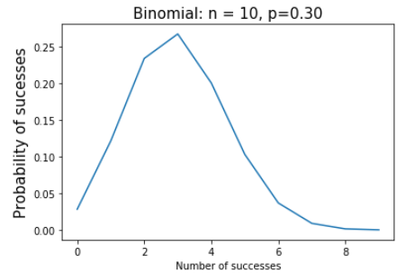
1.1 离散型随机变量-(伯努利分布):
from scipy.stats import binom
import matplotlib.pyplot as plt
import numpy as np
n = 10
p = 0.3
k = np.arange(0, 10)
binomial = binom.pmf(k, n, p)
plt.plot(k, binomial)
plt.title('Binomial: n = %i, p=%0.2f' % (n, p), fontsize=15)
plt.xlabel('Number of successes')
plt.ylabel('Probability of sucesses', fontsize=15)
plt.show()
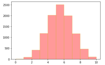
1.2 离散型随机变量-(二项分布):
dis_2 = np.random.binomial(10,0.5,size=10000)
plt.hist(dis_2,bins=10,color='r',alpha=0.4,edgecolor='y')
plt.show()
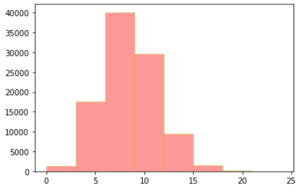
1.3 离散型随机变量-(泊松分布):
dis_3 = np.random.poisson(8,100000)
# lam随机事件发生率,size形状 n * p = 8
plt.hist(dis_3,bins=8,color='r',alpha=0.4,edgecolor='y')
plt.show()
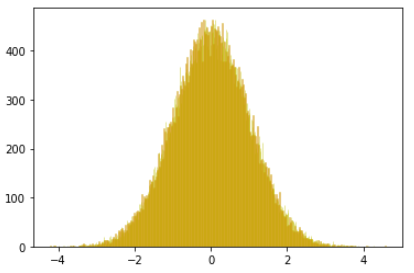
1.4 连续型随机变量-(正态分布):
dis_4 = np.random.normal(0,1,100000)
plt.hist(dis_4,bins=800,color='r',alpha=0.4,edgecolor='y')
plt.show()
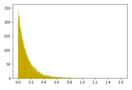
1.5 连续型随机变量-(指数分布):
dis_5 = np.random.exponential(0.125,100000)
plt.hist(dis_5,bins=6000,color='r',alpha=0.4,edgecolor='y')
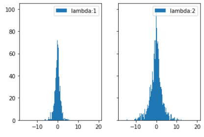
1.6 连续型随机变量-(拉普拉斯分布):
import numpy as np
laplace1 = np.random.laplace(0, 1, 10000)
laplace2 = np.random.laplace(0, 2, 10000)

import matplotlib.pyplot as plt
fig, (ax1, ax2) = plt.subplots(1,2, sharex=True, sharey=True)
ax1.hist(laplace1,bins=1000, label="lambda:1")
ax1.legend()

ax2.hist(laplace2, bins=1000, label="lambda:2")
ax2.legend()
plt.show()