本文主要解读CenterNet如何加载数据,并将标注信息转化为CenterNet规定的高斯分布的形式。
1. YOLOv3和CenterNet流程对比
CenterNet和Anchor-Based的方法不同,以YOLOv3为例,大致梳理一下模型的框架和数据处理流程。
YOLOv3是一个经典的单阶段的目标检测算法,图片进入网络的流程如下:
- 对图片进行resize,长和宽都要是32的倍数。
- 图片经过网络的特征提取后,空间分辨率变为原来的1/32。
- 得到的Tensor去代表图片不同尺度下的目标框,其中目标框的表示为(x,y,w,h,c),分别代表左上角坐标,宽和高,含有某物体的置信度。
- 训练完成后,测试的时候需要使用非极大抑制算法得到最终的目标框。
CenterNet是一个经典的Anchor-Free目标检测方法,图片进入网络流程如下:
- 对图片进行resize,长和宽一般相等,并且至少为4的倍数。
- 图片经过网络的特征提取后,得到的特征图的空间分辨率依然比较大,是原来的1/4。这是因为CenterNet采用的是类似人体姿态估计中用到的骨干网络,基于heatmap提取关键点的方法需要最终的空间分辨率比较大。
- 训练的过程中,CenterNet得到的是一个heatmap,所以标签加载的时候,需要转为类似的heatmap热图。
- 测试的过程中,由于只需要从热图中提取目标,这样就不需要使用NMS,降低了计算量。
2. CenterNet部分详解
设输入图片为(Iin R^{W imes H imes 3}), W代表图片的宽,H代表高。CenterNet的输出是一个关键点热图heatmap。
其中R代表输出的stride大小,C代表关键点的类型的个数。
举个例子,在COCO数据集目标检测中,R设置为4,C的值为80,代表80个类别。
如果(hat{Y}_{x,y,c}=1)代表检测到一个物体,表示对类别c来说,(x,y)这个位置检测到了c类的目标。
既然输出是热图,标签构建的ground truth也必须是热图的形式。标注的内容一般包含(x1,y1,x2,y2,c),目标框左上角坐标、右下角坐标和类别c,按照以下流程转为ground truth:
- 得到原图中对应的中心坐标(p=(frac{x1+x2}{2}, frac{y1+y2}{2}))
- 得到下采样后的feature map中对应的中心坐标( ilde{p}=lfloor frac{p}{R} floor), R代表下采样倍数,CenterNet中R为4
- 如果输入图片为512,那么输出的feature map的空间分辨率为[128x128], 将标注的目标框以高斯核的方式将关键点分布到特征图上:
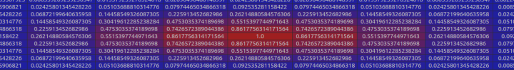
其中(sigma_p)是一个与目标大小相关的标准差(代码中设置的是)。对于特殊情况,相同类别的两个高斯分布发生了重叠,重叠元素间最大的值作为最终元素。下图是知乎用户OLDPAN分享的高斯分布图。
3. 代码部分
datasets/pascal.py 的代码主要从getitem函数入手,以下代码已经做了注释,其中最重要的两个部分一个是如何获取高斯半径(gaussian_radius函数),一个是如何将高斯分布分散到heatmap上(draw_umich_gaussian函数)。
def __getitem__(self, index):
    img_id = self.images[index]
    img_path = os.path.join(
        self.img_dir, self.coco.loadImgs(ids=[img_id])[0]['file_name'])
    ann_ids = self.coco.getAnnIds(imgIds=[img_id])
    annotations = self.coco.loadAnns(ids=ann_ids)

    labels = np.array([self.cat_ids[anno['category_id']]
                        for anno in annotations])
    bboxes = np.array([anno['bbox']
                        for anno in annotations], dtype=np.float32)

    if len(bboxes) == 0:
        bboxes = np.array([[0., 0., 0., 0.]], dtype=np.float32)
        labels = np.array([[0]])

    bboxes[:, 2:] += bboxes[:, :2]  # xywh to xyxy

    img = cv2.imread(img_path)
    height, width = img.shape[0], img.shape[1]
    # 获取中心坐标p
    center = np.array([width / 2., height / 2.],
                        dtype=np.float32)  # center of image
    scale = max(height, width) * 1.0  # 仿射变换

    flipped = False
    if self.split == 'train':
        # 随机选择一个尺寸来训练
        scale = scale * np.random.choice(self.rand_scales)
        w_border = get_border(128, width)
        h_border = get_border(128, height)
        center[0] = np.random.randint(low=w_border, high=width - w_border)
        center[1] = np.random.randint(low=h_border, high=height - h_border)

        if np.random.random() < 0.5:
            flipped = True
            img = img[:, ::-1, :]
            center[0] = width - center[0] - 1

    # 仿射变换
    trans_img = get_affine_transform(
        center, scale, 0, [self.img_size['w'], self.img_size['h']])
    img = cv2.warpAffine(
        img, trans_img, (self.img_size['w'], self.img_size['h']))

    # 归一化
    img = (img.astype(np.float32) / 255.)
    if self.split == 'train':
        # 对图片的亮度对比度等属性进行修改
        color_aug(self.data_rng, img, self.eig_val, self.eig_vec)

    img -= self.mean
    img /= self.std
    img = img.transpose(2, 0, 1)  # from [H, W, C] to [C, H, W]

    # 对Ground Truth heatmap进行仿射变换
    trans_fmap = get_affine_transform(
        center, scale, 0, [self.fmap_size['w'], self.fmap_size['h']]) # 这时候已经是下采样为原来的四分之一了

    # 3个最重要的变量
    hmap = np.zeros(
        (self.num_classes, self.fmap_size['h'], self.fmap_size['w']), dtype=np.float32)  # heatmap
    w_h_ = np.zeros((self.max_objs, 2), dtype=np.float32)  # width and height
    regs = np.zeros((self.max_objs, 2), dtype=np.float32)  # regression

    # indexs
    inds = np.zeros((self.max_objs,), dtype=np.int64)
    # 具体选择哪些index
    ind_masks = np.zeros((self.max_objs,), dtype=np.uint8)

    for k, (bbox, label) in enumerate(zip(bboxes, labels)):
        if flipped:
            bbox[[0, 2]] = width - bbox[[2, 0]] - 1

        # 对检测框也进行仿射变换
        bbox[:2] = affine_transform(bbox[:2], trans_fmap)
        bbox[2:] = affine_transform(bbox[2:], trans_fmap)
        # 防止越界
        bbox[[0, 2]] = np.clip(bbox[[0, 2]], 0, self.fmap_size['w'] - 1)
        bbox[[1, 3]] = np.clip(bbox[[1, 3]], 0, self.fmap_size['h'] - 1)
        # 得到高和宽
        h, w = bbox[3] - bbox[1], bbox[2] - bbox[0]

        if h > 0 and w > 0:
            obj_c = np.array([(bbox[0] + bbox[2]) / 2, (bbox[1] + bbox[3]) / 2],
                                dtype=np.float32) # 中心坐标-浮点型
            obj_c_int = obj_c.astype(np.int32) # 整型的中心坐标
            # 根据一元二次方程计算出最小的半径
            radius = max(0, int(gaussian_radius((math.ceil(h), math.ceil(w)), self.gaussian_iou)))
            # 得到高斯分布
            draw_umich_gaussian(hmap[label], obj_c_int, radius)

            w_h_[k] = 1. * w, 1. * h

            # 记录偏移量
            regs[k] = obj_c - obj_c_int  # discretization error
            # 当前是obj序列中的第k个 = fmap_w * cy + cx = fmap中的序列数
            inds[k] = obj_c_int[1] * self.fmap_size['w'] + obj_c_int[0]
            # 进行mask标记
            ind_masks[k] = 1

    return {'image': img, 'hmap': hmap, 'w_h_': w_h_, 'regs': regs,
            'inds': inds, 'ind_masks': ind_masks, 'c': center,
            's': scale, 'img_id': img_id}
4. heatmap上应用高斯核
heatmap上使用高斯核有很多需要注意的细节。CenterNet官方版本实际上是在CornerNet的基础上改动得到的,有很多祖传代码。
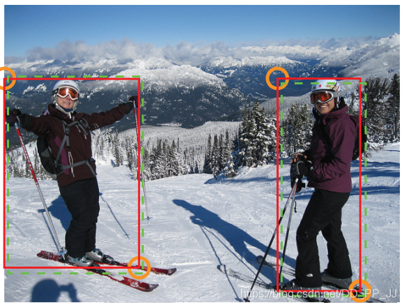
在使用高斯核前要考虑这样一个问题,下图来自于CornerNet论文中的图示,红色的是标注框,但绿色的其实也可以作为最终的检测结果保留下来。那么这个问题可以转化为绿框在红框多大范围以内可以被接受。使用IOU来衡量红框和绿框的贴合程度,当两者IOU>0.7的时候,认为绿框也可以被接受,反之则不被接受。
那么现在问题转化为,如何确定半径r, 让红框和绿框的IOU大于0.7。
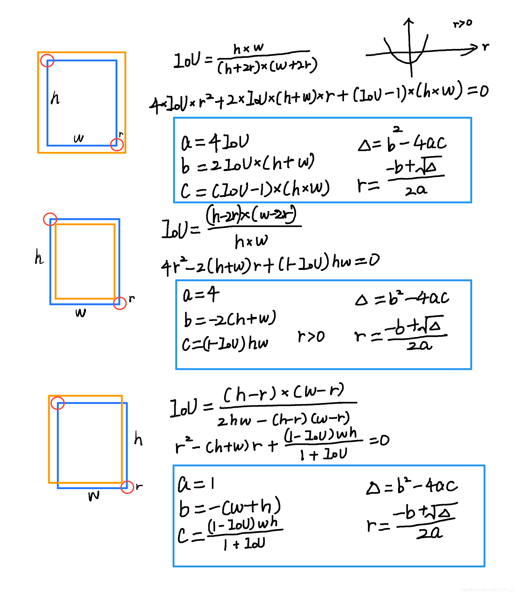
以上是三种情况,其中蓝框代表标注框,橙色代表可能满足要求的框。这个问题最终变为了一个一元二次方程有解的问题,同时由于半径必须为正数,所以r的取值就可以通过求根公式获得。
def gaussian_radius(det_size, min_overlap=0.7):
    # gt框的长和宽
    height, width = det_size

    a1 = 1
    b1 = (height + width)
    c1 = width * height * (1 - min_overlap) / (1 + min_overlap)
    sq1 = np.sqrt(b1 ** 2 - 4 * a1 * c1)
    r1 = (b1 + sq1) / (2 * a1)

    a2 = 4
    b2 = 2 * (height + width)
    c2 = (1 - min_overlap) * width * height
    sq2 = np.sqrt(b2 ** 2 - 4 * a2 * c2)
    r2 = (b2 + sq2) / (2 * a2)

    a3 = 4 * min_overlap
    b3 = -2 * min_overlap * (height + width)
    c3 = (min_overlap - 1) * width * height
    sq3 = np.sqrt(b3 ** 2 - 4 * a3 * c3)
    r3 = (b3 + sq3) / (2 * a3)

    return min(r1, r2, r3)
可以看到这里的公式和上图计算的结果是一致的,需要说明的是,CornerNet最开始版本中这里出现了错误,分母不是2a,而是直接设置为2。CenterNet也延续了这个bug,CenterNet作者回应说这个bug对结果的影响不大,但是根据issue的讨论来看,有一些人通过修正这个bug以后,可以让AR提升1-3个百分点。以下是有bug的版本,CornerNet最新版中已经修复了这个bug。
def gaussian_radius(det_size, min_overlap=0.7):
  height, width = det_size

  a1  = 1
  b1  = (height + width)
  c1  = width * height * (1 - min_overlap) / (1 + min_overlap)
  sq1 = np.sqrt(b1 ** 2 - 4 * a1 * c1)
  r1  = (b1 + sq1) / 2

  a2  = 4
  b2  = 2 * (height + width)
  c2  = (1 - min_overlap) * width * height
  sq2 = np.sqrt(b2 ** 2 - 4 * a2 * c2)
  r2  = (b2 + sq2) / 2

  a3  = 4 * min_overlap
  b3  = -2 * min_overlap * (height + width)
  c3  = (min_overlap - 1) * width * height
  sq3 = np.sqrt(b3 ** 2 - 4 * a3 * c3)
  r3  = (b3 + sq3) / 2

  return min(r1, r2, r3)
同时有一些人认为圆并不普适,提出了使用椭圆来进行计算,也有人在issue中给出了推导,感兴趣的可以看以下链接:https://github.com/princeton-vl/CornerNet/issues/110
5. 高斯分布添加到heatmap上
def gaussian2D(shape, sigma=1):
    m, n = [(ss - 1.) / 2. for ss in shape]
    y, x = np.ogrid[-m:m + 1, -n:n + 1]

    h = np.exp(-(x * x + y * y) / (2 * sigma * sigma))
    h[h < np.finfo(h.dtype).eps * h.max()] = 0
    # 限制最小的值
    return h

def draw_umich_gaussian(heatmap, center, radius, k=1):
    # 得到直径
    diameter = 2 * radius + 1
    gaussian = gaussian2D((diameter, diameter), sigma=diameter / 6)
    # sigma是一个与直径相关的参数
    # 一个圆对应内切正方形的高斯分布

    x, y = int(center[0]), int(center[1])

    height, width = heatmap.shape[0:2]

    # 对边界进行约束,防止越界
    left, right = min(x, radius), min(width - x, radius + 1)
    top, bottom = min(y, radius), min(height - y, radius + 1)

    # 选择对应区域
    masked_heatmap = heatmap[y - top:y + bottom, x - left:x + right]
    # 将高斯分布结果约束在边界内
    masked_gaussian = gaussian[radius - top:radius + bottom,
                               radius - left:radius + right]

    if min(masked_gaussian.shape) > 0 and min(masked_heatmap.shape) > 0:  # TODO debug
        np.maximum(masked_heatmap, masked_gaussian * k, out=masked_heatmap)
        # 将高斯分布覆盖到heatmap上,相当于不断的在heatmap基础上添加关键点的高斯,
        # 即同一种类型的框会在一个heatmap某一个类别通道上面上面不断添加。
        # 最终通过函数总体的for循环,相当于不断将目标画到heatmap
    return heatmap
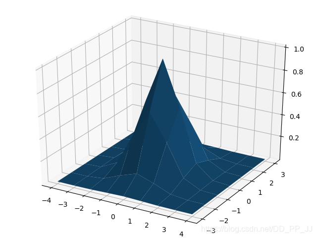
使用matplotlib对gaussian2D进行可视化。
import numpy as np
y,x = np.ogrid[-4:5,-3:4]
sigma = 1
h=np.exp(-(x*x+y*y)/(2*sigma*sigma))
import matplotlib.pyplot as plt
from mpl_toolkits.mplot3d import Axes3D
fig = plt.figure()
ax = Axes3D(fig)
ax.plot_surface(x,y,h)
plt.show()
6. 参考
[1]https://zhuanlan.zhihu.com/p/66048276
[2]https://www.cnblogs.com/shine-lee/p/9671253.html
[3]https://zhuanlan.zhihu.com/p/96856635