【GiantPandaCV导语】CoAt=Convolution + Attention,paperwithcode榜单第一名,通过结合卷积与Transformer实现性能上的突破,方法部分设计非常规整,层层深入考虑模型的架构设计。

引言
Transformer模型的容量大,由于缺乏正确的归纳偏置,泛化能力要比卷积网络差。
提出了CoAtNets模型族:
- 深度可分离卷积与self-attention能够通过简单的相对注意力来统一化。
- 叠加卷积层和注意层在提高泛化能力和效率方面具有惊人的效果
方法
这部分主要关注如何将conv与transformer以一种最优的方式结合:
- 在基础的计算块中,如果合并卷积与自注意力操作。
- 如何组织不同的计算模块来构建整个网络。
合并卷积与自注意力
卷积方面谷歌使用的是经典的MBConv, 使用深度可分离卷积来捕获空间之间的交互。
卷积操作的表示:\(\mathcal{L}(i)\)代表i周边的位置,也即卷积处理的感受野。
自注意力表示:\(\mathcal{G}\)表示全局空间感受野。
融合方法一:先求和,再softmax
融合方法二:先softmax,再求和
出于参数量、计算两方面的考虑,论文打算采用第二种融合方法。
垂直布局设计
决定好合并卷积与注意力的方式后应该考虑如何构建网络整体架构,主要有三个方面的考量:
- 使用降采样降低空间维度大小,然后使用global relative attention。
- 使用局部注意力,强制全局感受野限制在一定范围内。典型代表有:
- Scaling local self-attention for parameter efficient visual backbone
- Swin Transformer
- 使用某种线性注意力方法来取代二次的softmax attention。典型代表有:
- Efficient Attention
- Transformers are rnns
- Rethinking attention with performers
第二种方法实现效率不够高,第三种方法性能不够好,因此采用第一种方法,如何设计降采样的方式也有几种方案:
- 使用卷积配合stride进行降采样。
- 使用pooling操作完成降采样,构建multi-stage网络范式。
- 根据第一种方案提出\(ViT_{REL}\), 即使用ViT Stem,直接堆叠L层Transformer block使用relative attention。
- 根据第二种方案,采用multi-stage方案提出模型组:\(S_0,...,S_4\),如下图所示:
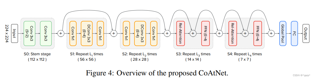
\(S_o-S_2\)采用卷积以及MBConv,从\(S_2-S_4\)的几个模块采用Transformer 结构。具体Transformer内部有以下几个变体:C代表卷积,T代表Transformer
- C-C-C-C
- C-C-C-T
- C-C-T-T
- C-T-T-T
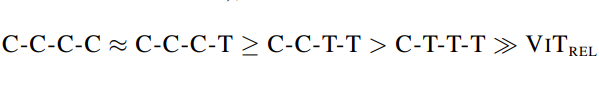
初步测试模型泛化能力
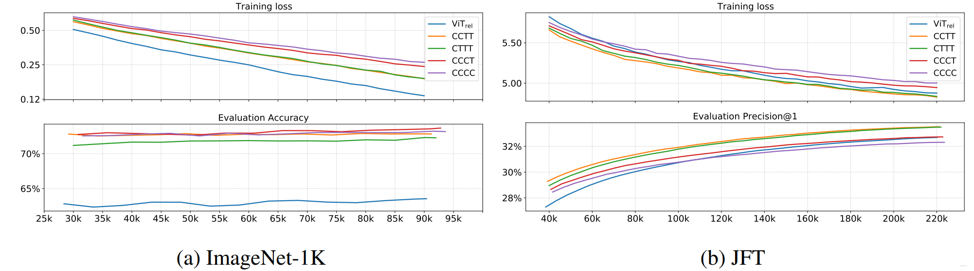
泛化能力排序为:(证明架构中还是需要存在想当比例的卷积操作)
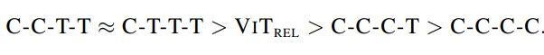
初步测试模型容量
主要是从JFT以及ImageNet-1k上不同的表现来判定的,排序结果为:
测试模型迁移能力
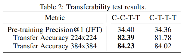
为了进一步比较CCTT与CTTT,进行了迁移能力测试,发现CCTT能够超越CTTT。
最终CCTT胜出!
实验
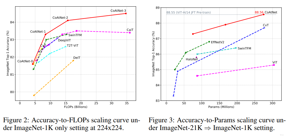
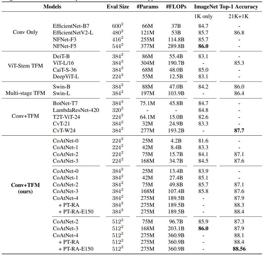
与SOTA模型比较结果:
实验结果:
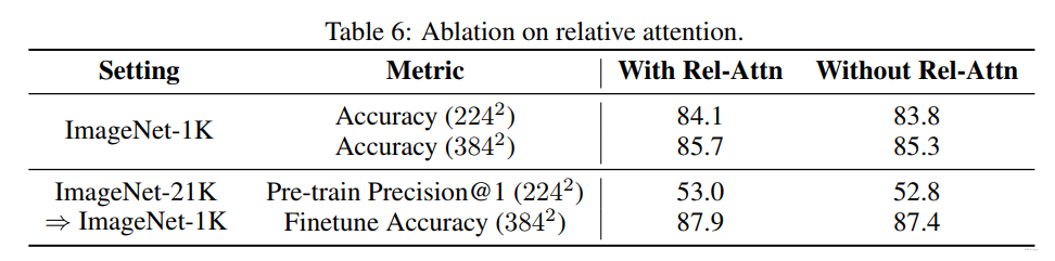
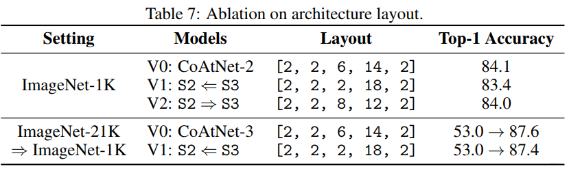
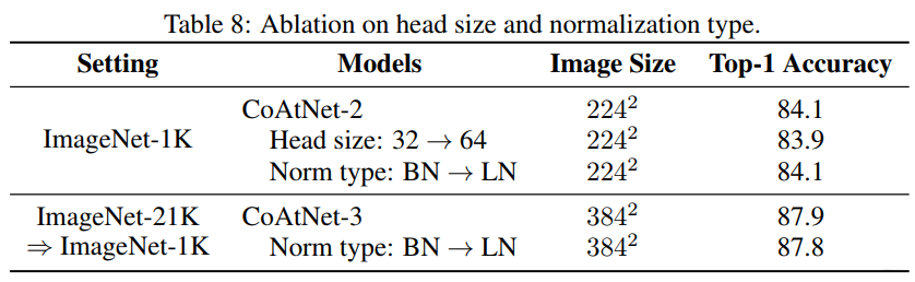
消融实验:
代码
浅层使用的MBConv模块如下:
class MBConv(nn.Module):
    def __init__(self, inp, oup, image_size, downsample=False, expansion=4):
        super().__init__()
        self.downsample = downsample
        stride = 1 if self.downsample == False else 2
        hidden_dim = int(inp * expansion)

        if self.downsample:
            self.pool = nn.MaxPool2d(3, 2, 1)
            self.proj = nn.Conv2d(inp, oup, 1, 1, 0, bias=False)

        if expansion == 1:
            self.conv = nn.Sequential(
                # dw
                nn.Conv2d(hidden_dim, hidden_dim, 3, stride,
                          1, groups=hidden_dim, bias=False),
                nn.BatchNorm2d(hidden_dim),
                nn.GELU(),
                # pw-linear
                nn.Conv2d(hidden_dim, oup, 1, 1, 0, bias=False),
                nn.BatchNorm2d(oup),
            )
        else:
            self.conv = nn.Sequential(
                # pw
                # down-sample in the first conv
                nn.Conv2d(inp, hidden_dim, 1, stride, 0, bias=False),
                nn.BatchNorm2d(hidden_dim),
                nn.GELU(),
                # dw
                nn.Conv2d(hidden_dim, hidden_dim, 3, 1, 1,
                          groups=hidden_dim, bias=False),
                nn.BatchNorm2d(hidden_dim),
                nn.GELU(),
                SE(inp, hidden_dim),
                # pw-linear
                nn.Conv2d(hidden_dim, oup, 1, 1, 0, bias=False),
                nn.BatchNorm2d(oup),
            )

        self.conv = PreNorm(inp, self.conv, nn.BatchNorm2d)

    def forward(self, x):
        if self.downsample:
            return self.proj(self.pool(x)) + self.conv(x)
        else:
            return x + self.conv(x)
主要关注Attention Block设计,引入Relative Position:
class Attention(nn.Module):
    def __init__(self, inp, oup, image_size, heads=8, dim_head=32, dropout=0.):
        super().__init__()
        inner_dim = dim_head * heads
        project_out = not (heads == 1 and dim_head == inp)

        self.ih, self.iw = image_size

        self.heads = heads
        self.scale = dim_head ** -0.5

        # parameter table of relative position bias
        self.relative_bias_table = nn.Parameter(
            torch.zeros((2 * self.ih - 1) * (2 * self.iw - 1), heads))

        coords = torch.meshgrid((torch.arange(self.ih), torch.arange(self.iw)))
        coords = torch.flatten(torch.stack(coords), 1)
        relative_coords = coords[:, :, None] - coords[:, None, :]

        relative_coords[0] += self.ih - 1
        relative_coords[1] += self.iw - 1
        relative_coords[0] *= 2 * self.iw - 1
        relative_coords = rearrange(relative_coords, 'c h w -> h w c')
        relative_index = relative_coords.sum(-1).flatten().unsqueeze(1)
        self.register_buffer("relative_index", relative_index)

        self.attend = nn.Softmax(dim=-1)
        self.to_qkv = nn.Linear(inp, inner_dim * 3, bias=False)

        self.to_out = nn.Sequential(
            nn.Linear(inner_dim, oup),
            nn.Dropout(dropout)
        ) if project_out else nn.Identity()

    def forward(self, x):
        qkv = self.to_qkv(x).chunk(3, dim=-1)
        q, k, v = map(lambda t: rearrange(
            t, 'b n (h d) -> b h n d', h=self.heads), qkv)

        dots = torch.matmul(q, k.transpose(-1, -2)) * self.scale

        # Use "gather" for more efficiency on GPUs
        relative_bias = self.relative_bias_table.gather(
            0, self.relative_index.repeat(1, self.heads))
        relative_bias = rearrange(
            relative_bias, '(h w) c -> 1 c h w', h=self.ih*self.iw, w=self.ih*self.iw)
        dots = dots + relative_bias

        attn = self.attend(dots)
        out = torch.matmul(attn, v)
        out = rearrange(out, 'b h n d -> b n (h d)')
        out = self.to_out(out)
        return out