TensorFlow新手必学篇【理论+实战】

1：你想要学习TensorFlow，首先你得安装Tensorflow，在你学习的时候你最好懂以下的知识：
    a：怎么用python编程；
     b：了解一些关于数组的知识；
     c：最理想的情况是：关于机器学习，懂一点点；或者不懂也是可以慢慢开始学习的。

2：TensorFlow提供很多API，最低级别是API:TensorFlow Core，提供给你完成程序控制,还有一些高级别的API，它们是构建在
TensorFlow Core之上的，这些高级别的API更加容易学习和使用，于此同时，这些高级别的API使得重复的训练任务更加容易，
也使得多个使用者操作对他保持一致性，一个高级别的API像tf.estimator帮助你管理数据集合，估量，训练和推理。

3：TensorsTensorFlow的数据中央控制单元是tensor(张量)，一个tensor由一系列的原始值组成，这些值被形成一个任意维数的数组。
一个tensor的列就是它的维度。

4：
import tensorflow as tf
上面的是TensorFlow 程序典型的导入语句，作用是：赋予Python访问TensorFlow类(classes)，方法（methods），符号(symbols)

5：The Computational Graph TensorFlow核心程序由2个独立部分组成：
    a:Building the computational graph构建计算图
    b:Running the computational graph运行计算图
一个computational graph(计算图)是一系列的TensorFlow操作排列成一个节点图。

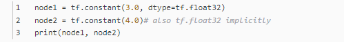
 最后打印结果是：

Tensor("Const:0", shape=(), dtype=float32) Tensor("Const_1:0",shape=(), dtype=float32)

要想打印最终结果，我们必须用到session:一个session封装了TensorFlow运行时的控制和状态

 我们可以组合Tensor节点操作(操作仍然是一个节点)来构造更加复杂的计算，

 打印结果是：

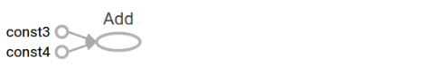
 6：TensorFlow提供一个统一的调用称之为TensorBoard，它能展示一个计算图的图片；如下面这个截图就展示了这个计算图

 7：一个计算图可以参数化的接收外部的输入，作为一个placeholders(占位符)，一个占位符是允许后面提供一个值的。

里有点像一个function (函数)或者lambda表达式，我们定义了2个输入参数a和b，然后提供一个在它们之上的操作。我们可以使用

feed_dict(传递字典)参数传递具体的值到run方法的占位符来进行多个输入，从而来计算这个图。

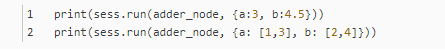
 结果是：

在TensorBoard，计算图类似于这样：

 

 8：我们可以增加另外的操作来让计算图更加复杂，比如

 在TensorBoard，计算图类似于这样：

 9：在机器学习中，我们通常想让一个模型可以接收任意多个输入，比如大于1个，好让这个模型可以被训练，在不改变输入的情况下,

我们需要改变这个计算图去获得一个新的输出。变量允许我们增加可训练的参数到这个计算图中，它们被构造成有一个类型和初始值：

 10：当你调用tf.constant时常量被初始化，它们的值是不可以改变的，而变量当你调用tf.Variable时没有被初始化，

在TensorFlow程序中要想初始化这些变量，你必须明确调用一个特定的操作，如下：

 11：要实现初始化所有全局变量的TensorFlow子图的的处理是很重要的，直到我们调用sess.run，这些变量都是未被初始化的。

既然x是一个占位符，我们就可以同时地对多个x的值进行求值linear_model，例如：

 12：我们已经创建了一个模型，但是我们至今不知道它是多好，在这些训练数据上对这个模型进行评估，我们需要一个

y占位符来提供一个期望的值，并且我们需要写一个loss function(损失函数)，一个损失函数度量当前的模型和提供

的数据有多远，我们将会使用一个标准的损失模式来线性回归，它的增量平方和就是当前模型与提供的数据之间的损失

，linear_model - y创建一个向量，其中每个元素都是对应的示例错误增量。这个错误的方差我们称为tf.square。然后

，我们合计所有的错误方差用以创建一个标量，用tf.reduce_sum抽象出所有示例的错误。

13：我们分配一个值给W和b(得到一个完美的值是-1和1)来手动改进这一点,一个变量被初始化一个值会调用tf.Variable，

但是可以用tf.assign来改变这个值，例如：fixW = tf.assign(W, [-1.])

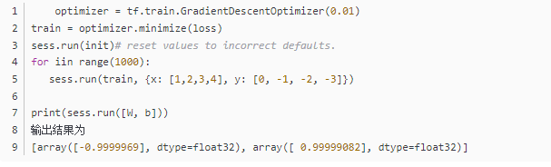
14：tf.train APITessorFlow提供optimizers(优化器)，它能慢慢改变每一个变量以最小化损失函数，最简单的优化器是

gradient descent(梯度下降)，它根据变量派生出损失的大小,来修改每个变量。通常手工计算变量符号是乏味且容易出错的，

因此，TensorFlow使用函数tf.gradients给这个模型一个描述，从而能自动地提供衍生品，简而言之，优化器通常会为你做这个。例如：

现在你已经完成了实际的机器学习，尽管这个简单的线性回归模型不要求太多TensorFlow core代码，更复杂的模型和

方法将数据输入到模型中，需要跟多的代码，因此TensorFlow为常见模式，结构和功能提供更高级别的抽象，我们将会

在下一个章节学习这些抽象。

15：tf.estimatortf.setimator是一个更高级别的TensorFlow库，它简化了机械式的机器学习，包含以下几个方面：

running training loops 运行训练循环

running evaluation loops 运行求值循环

managing data sets 管理数据集合

tf.setimator定义了很多相同的模型。

 

16：A custom modeltf.setimator没有把你限制在预定好的模型中，假设我们想要创建一个自定义的模型，它不是由

TensorFlow建成的。我还是能保持这些数据集合，输送，训练高级别的抽象；例如：tf.estimator;

 

17：现在你有了关于TensorFlow的一个基本工作知识，我们还有更多教程，它能让你学习更多。如果你是一个机器学习初学者，

你可以继续学习MNIST for beginners，否则你可以学习Deep MNIST for experts.

   如果还有问题未能得到解决，搜索887934385交流群，进入后下载资料工具安装包等。最后，感谢观看！

完整的代码：

import tensorflow as tf

node1 = tf.constant(3.0, dtype=tf.float32)

node2 = tf.constant(4.0)  # also tf.float32 implicitly

print(node1, node2)

 

sess = tf.Session()

print(sess.run([node1, node2]))

 

# from __future__ import print_function

node3 = tf.add(node1, node2)

print("node3:", node3)

print("sess.run(node3):", sess.run(node3))

 

 

# 占位符

a = tf.placeholder(tf.float32)

b = tf.placeholder(tf.float32)

adder_node = a + b  # + provides a shortcut for tf.add(a, b)

 

print(sess.run(adder_node, {a: 3, b: 4.5}))

print(sess.run(adder_node, {a: [1, 3], b: [2, 4]}))

 

add_and_triple = adder_node * 3.

print(sess.run(add_and_triple, {a: 3, b: 4.5}))

 

 

# 多个变量求值

W = tf.Variable([.3], dtype=tf.float32)

b = tf.Variable([-.3], dtype=tf.float32)

x = tf.placeholder(tf.float32)

linear_model = W*x + b

 

#  变量初始化

init = tf.global_variables_initializer()

sess.run(init)

 

print(sess.run(linear_model, {x: [1, 2, 3, 4]}))

 

# loss function

y = tf.placeholder(tf.float32)

squared_deltas = tf.square(linear_model - y)

loss = tf.reduce_sum(squared_deltas)

print("loss function", sess.run(loss, {x: [1, 2, 3, 4], y: [0, -1, -2, -3]}))

 

ss = (0-0)*(0-0) + (0.3+1)*(0.3+1) + (0.6+2)*(0.6+2) + (0.9+3)*(0.9+3)  # 真实算法

print("真实算法ss", ss)

 

print(sess.run(loss, {x: [1, 2, 3, 4], y: [0, 0.3, 0.6, 0.9]}))  # 测试参数

 

# ft.assign 变量重新赋值

fixW = tf.assign(W, [-1.])

fixb = tf.assign(b, [1.])

sess.run([fixW, fixb])

print(sess.run(linear_model, {x: [1, 2, 3, 4]}))

print(sess.run(loss, {x: [1, 2, 3, 4], y: [0, -1, -2, -3]}))

 

 

# tf.train API

optimizer = tf.train.GradientDescentOptimizer(0.01)  # 梯度下降优化器

train = optimizer.minimize(loss)    # 最小化损失函数

sess.run(init)  # reset values to incorrect defaults.

for i in range(1000):

  sess.run(train, {x: [1, 2, 3, 4], y: [0, -1, -2, -3]})

 

print(sess.run([W, b]))

 

 

print("------------------------------------1")

 

# Complete program:The completed trainable linear regression model is shown here:完整的训练线性回归模型代码

# Model parameters

W = tf.Variable([.3], dtype=tf.float32)

b = tf.Variable([-.3], dtype=tf.float32)

# Model input and output

x = tf.placeholder(tf.float32)

linear_model = W*x + b

y = tf.placeholder(tf.float32)

 

# loss

loss = tf.reduce_sum(tf.square(linear_model - y))  # sum of the squares

# optimizer

optimizer = tf.train.GradientDescentOptimizer(0.01)

train = optimizer.minimize(loss)

 

# training data

x_train = [1, 2, 3, 4]

y_train = [0, -1, -2, -3]

# training loop

init = tf.global_variables_initializer()

sess = tf.Session()

sess.run(init) # reset values to wrong

for i in range(1000):

  sess.run(train, {x: x_train, y: y_train})

 

# evaluate training accuracy

curr_W, curr_b, curr_loss = sess.run([W, b, loss], {x: x_train, y: y_train})

print("W: %s b: %s loss: %s"%(curr_W, curr_b, curr_loss))

 

 

print("------------------------------------2")

 

# tf.estimator  使用tf.estimator实现上述训练

# Notice how much simpler the linear regression program becomes with tf.estimator:

# NumPy is often used to load, manipulate and preprocess data.

import numpy as np

import tensorflow as tf

 

# Declare list of features. We only have one numeric feature. There are many

# other types of columns that are more complicated and useful.

feature_columns = [tf.feature_column.numeric_column("x", shape=[1])]

 

# An estimator is the front end to invoke training (fitting) and evaluation

# (inference). There are many predefined types like linear regression,

# linear classification, and many neural network classifiers and regressors.

# The following code provides an estimator that does linear regression.

estimator = tf.estimator.LinearRegressor(feature_columns=feature_columns)

 

# TensorFlow provides many helper methods to read and set up data sets.

# Here we use two data sets: one for training and one for evaluation

# We have to tell the function how many batches

# of data (num_epochs) we want and how big each batch should be.

x_train = np.array([1., 2., 3., 4.])

y_train = np.array([0., -1., -2., -3.])

x_eval = np.array([2., 5., 8., 1.])

y_eval = np.array([-1.01, -4.1, -7, 0.])

input_fn = tf.estimator.inputs.numpy_input_fn(

    {"x": x_train}, y_train, batch_size=4, num_epochs=None, shuffle=True)

train_input_fn = tf.estimator.inputs.numpy_input_fn(

    {"x": x_train}, y_train, batch_size=4, num_epochs=1000, shuffle=False)

eval_input_fn = tf.estimator.inputs.numpy_input_fn(

    {"x": x_eval}, y_eval, batch_size=4, num_epochs=1000, shuffle=False)

 

# We can invoke 1000 training steps by invoking the  method and passing the

# training data set.

estimator.train(input_fn=input_fn, steps=1000)

 

# Here we evaluate how well our model did.

train_metrics = estimator.evaluate(input_fn=train_input_fn)

eval_metrics = estimator.evaluate(input_fn=eval_input_fn)

print("train metrics: %r"% train_metrics)

print("eval metrics: %r"% eval_metrics)

 

 

print("------------------------------------3")

 

# A custom model：客户自定义实现训练

# Declare list of features, we only have one real-valued feature

def model_fn(features, labels, mode):

  # Build a linear model and predict values

  W = tf.get_variable("W", [1], dtype=tf.float64)

  b = tf.get_variable("b", [1], dtype=tf.float64)

  y = W*features['x'] + b

  # Loss sub-graph

  loss = tf.reduce_sum(tf.square(y - labels))

  # Training sub-graph

  global_step = tf.train.get_global_step()

  optimizer = tf.train.GradientDescentOptimizer(0.01)

  train = tf.group(optimizer.minimize(loss),

                   tf.assign_add(global_step, 1))

  # EstimatorSpec connects subgraphs we built to the

  # appropriate functionality.

  return tf.estimator.EstimatorSpec(

      mode=mode,

      predictions=y,

      loss=loss,

      train_op=train)

 

estimator = tf.estimator.Estimator(model_fn=model_fn)

# define our data sets

x_train = np.array([1., 2., 3., 4.])

y_train = np.array([0., -1., -2., -3.])

x_eval = np.array([2., 5., 8., 1.])

y_eval = np.array([-1.01, -4.1, -7., 0.])

input_fn = tf.estimator.inputs.numpy_input_fn(

    {"x": x_train}, y_train, batch_size=4, num_epochs=None, shuffle=True)

train_input_fn = tf.estimator.inputs.numpy_input_fn(

    {"x": x_train}, y_train, batch_size=4, num_epochs=1000, shuffle=False)

eval_input_fn = tf.estimator.inputs.numpy_input_fn(

    {"x": x_eval}, y_eval, batch_size=4, num_epochs=1000, shuffle=False)

 

# train

estimator.train(input_fn=input_fn, steps=1000)

# Here we evaluate how well our model did.

train_metrics = estimator.evaluate(input_fn=train_input_fn)

eval_metrics = estimator.evaluate(input_fn=eval_input_fn)

print("train metrics: %r"% train_metrics)

 

print("eval metrics: %r"% eval_metrics)