5 建立基础模型,尝试多种算法
#之前把精力都放在了前面了,这回我的重点就要放在建模上了,导入所需要的包
# 数据分析库
import pandas as pd
import numpy as np

# warnings:警告——>忽视
pd.options.mode.chained_assignment = None
pd.set_option('display.max_columns', 60)

# 可视化
import matplotlib.pyplot as plt
%matplotlib inline

# 字体大小设置
plt.rcParams['font.size'] = 24

from IPython.core.pylabtools import figsize

# Seaborn 高级可视化工具
import seaborn as sns
sns.set(font_scale = 2)

# 预处理:缺失值 、 最大最小归一化
from sklearn.preprocessing import Imputer, MinMaxScaler

# 机器学习算法库
from sklearn.linear_model import LinearRegression
from sklearn.ensemble import RandomForestRegressor, GradientBoostingRegressor
from sklearn.svm import SVR
from sklearn.neighbors import KNeighborsRegressor

# 调参工具包
from sklearn.model_selection import RandomizedSearchCV, GridSearchCV


import warnings
warnings.filterwarnings("ignore")
- 上次保存好的数据加载进来
# Read in data into dataframes
train_features = pd.read_csv('data/training_features.csv')
test_features = pd.read_csv('data/testing_features.csv')
train_labels = pd.read_csv('data/training_labels.csv')
test_labels = pd.read_csv('data/testing_labels.csv')

# Display sizes of data
print('Training Feature Size: ', train_features.shape)
print('Testing Feature Size:  ', test_features.shape)
print('Training Labels Size:  ', train_labels.shape)
print('Testing Labels Size:   ', test_labels.shape)
Training Feature Size:  (6622, 67)
Testing Feature Size:   (2839, 67)
Training Labels Size:   (6622, 1)
Testing Labels Size:    (2839, 1)
train_features.head()
5.1 缺失值填充

imputer = Imputer(strategy='median') # 因为数据有离群点,有大有小,用mean不太合适,用中位数较合适
# 在训练特征中训练
imputer.fit(train_features)

# 对训练数据进行转换
X = imputer.transform(train_features)#用中位数来代替做成的训练集
X_test = imputer.transform(test_features) #用中位数来代替做成的测试集
#np.isnan:数值进行空值检测
print('Missing values in training features: ', np.sum(np.isnan(X))) #返回的是0 ,代表缺失值任务已经完成了
print('Missing values in testing features:  ', np.sum(np.isnan(X_test)))
Missing values in training features:  0
Missing values in testing features:   0
5.2 特征进行与归一化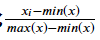
scaler = MinMaxScaler(feature_range=(0, 1))

# 训练与转换
scaler.fit(X)

# 把训练数据转换过来(0,1)
X = scaler.transform(X)
X_test = scaler.transform(X_test) # 测试数据
#标签值是1列 ,reshape变成1行
# reshape(行数,列数)常用来更改数据的行列数目
y = np.array(train_labels).reshape((-1,))#一维数组 , 变成1列
y_test = np.array(test_labels).reshape((-1, )) # 一维数组 , 变成1列
6 建立基础模型,尝试多种算法(回归问题)
1. Linear Regression
2. Support Vector Machine Regression
3. Random Forest Regression
4. Gradient Boosting Regression
5. K-Nearest Neighbors Regression
6.1 建立损失函数

# 在这里的损失函数是MAE ,abs()是绝对值
def mae(y_true, y_pred):
    return np.mean(abs(y_true - y_pred))


#制作一个模型 ,训练模型和在验证集上验证模型的参数
def fit_and_evaluate(model):

    # 训练模型
    model.fit(X, y)

    # 训练模型开始在测试数据上训练
    model_pred = model.predict(X_test)
    model_mae = mae(y_test, model_pred)


    return model_mae
6.2 选择机器学习算法

lr = LinearRegression()#线性回归
lr_mae = fit_and_evaluate(lr)

print('Linear Regression Performance on the test set: MAE = %0.4f' % lr_mae)
Linear Regression Performance on the test set: MAE = 12.9817
svm = SVR(C = 1000, gamma = 0.1) #支持向量机
svm_mae = fit_and_evaluate(svm)

print('Support Vector Machine Regression Performance on the test set: MAE = %0.4f' % svm_mae)
Support Vector Machine Regression Performance on the test set: MAE = 10.9336
random_forest = RandomForestRegressor(random_state=60)#集成算法的随机森林
random_forest_mae = fit_and_evaluate(random_forest)

print('Random Forest Regression Performance on the test set: MAE = %0.4f' % random_forest_mae)
Random Forest Regression Performance on the test set: MAE = 10.0941
gradient_boosted = GradientBoostingRegressor(random_state=60) #梯度提升树
gradient_boosted_mae = fit_and_evaluate(gradient_boosted)

print('Gradient Boosted Regression Performance on the test set: MAE = %0.4f' % gradient_boosted_mae)
Gradient Boosted Regression Performance on the test set: MAE = 9.9893
knn = KNeighborsRegressor(n_neighbors=10)#K近邻算法
knn_mae = fit_and_evaluate(knn)

print('K-Nearest Neighbors Regression Performance on the test set: MAE = %0.4f' % knn_mae)
K-Nearest Neighbors Regression Performance on the test set: MAE = 12.6722
plt.style.use('fivethirtyeight')
figsize(8, 6)


model_comparison = pd.DataFrame({'model': ['Linear Regression', 'Support Vector Machine',
                                           'Random Forest', 'Gradient Boosted',
                                            'K-Nearest Neighbors'],
                                 'mae': [lr_mae, svm_mae, random_forest_mae,
                                         gradient_boosted_mae, knn_mae]})

#         ascending=True是对的意思升序      降序 :从大到小/从第1行到第5行    barh:横着去画的直方图
model_comparison.sort_values('mae', ascending = False).plot(x = 'model', y = 'mae', kind = 'barh',
                                                           color = 'red', edgecolor = 'black')

# 纵轴是算法模型的名称    yticks:为递增值向量       横轴是MAE损失                 xticks:为递增值向量
plt.ylabel(''); plt.yticks(size = 14); plt.xlabel('Mean Absolute Error'); plt.xticks(size = 14)
plt.title('Model Comparison on Test MAE', size = 20);

7 模型调参
7.1 调参

loss = ['ls', 'lad', 'huber']

# 所使用的弱“学习者”(决策树)的数量
n_estimators = [100, 500, 900, 1100, 1500]

# 决策树的最大深度
max_depth = [2, 3, 5, 10, 15]

# 决策树的叶节点所需的最小示例个数
min_samples_leaf = [1, 2, 4, 6, 8]

# 分割决策树节点所需的最小示例个数
min_samples_split = [2, 4, 6, 10]


hyperparameter_grid = {'loss': loss,
                       'n_estimators': n_estimators,
                       'max_depth': max_depth,
                       'min_samples_leaf': min_samples_leaf,
                       'min_samples_split': min_samples_split}

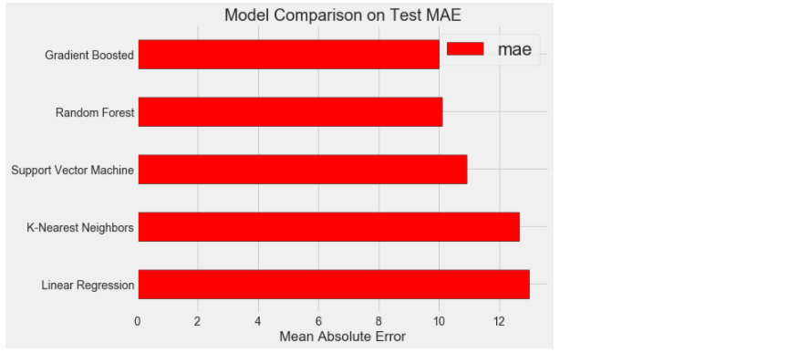
model = GradientBoostingRegressor(random_state = 42)


random_cv = RandomizedSearchCV(estimator=model,

                               param_distributions=hyperparameter_grid,
                               cv=4, n_iter=25,
                               scoring = 'neg_mean_absolute_error', #选择好结果的评估值

                               n_jobs = -1, verbose = 1,

                               return_train_score = True,

                               random_state=42)
# 注意:运行的时间非常慢,需要14mins
random_cv.fit(X, y)
RandomizedSearchCV(cv=4, error_score='raise-deprecating',
                   estimator=GradientBoostingRegressor(alpha=0.9,
                                                       criterion='friedman_mse',
                                                       init=None,
                                                       learning_rate=0.1,
                                                       loss='ls', max_depth=3,
                                                       max_features=None,
                                                       max_leaf_nodes=None,
                                                       min_impurity_decrease=0.0,
                                                       min_impurity_split=None,
                                                       min_samples_leaf=1,
                                                       min_samples_split=2,
                                                       min_weight_fraction_leaf=0.0,
                                                       n_estimators=100,...
                                                       verbose=0,
                                                       warm_start=False),
                   iid='warn', n_iter=25, n_jobs=-1,
                   param_distributions={'loss': ['ls', 'lad', 'huber'],
                                        'max_depth': [2, 3, 5, 10, 15],
                                        'min_samples_leaf': [1, 2, 4, 6, 8],
                                        'min_samples_split': [2, 4, 6, 10],
                                        'n_estimators': [100, 500, 900, 1100,
                                                         1500]},
                   pre_dispatch='2*n_jobs', random_state=42, refit=True,
                   return_train_score=True, scoring='neg_mean_absolute_error',
                   verbose=1)
random_cv.best_estimator_ #最好的参数
输出:GradientBoostingRegressor(alpha=0.9, criterion='friedman_mse', init=None,
                          learning_rate=0.1, loss='lad', max_depth=5,
                          max_features=None, max_leaf_nodes=None,
                          min_impurity_decrease=0.0, min_impurity_split=None,
                          min_samples_leaf=4, min_samples_split=2,
                          min_weight_fraction_leaf=0.0, n_estimators=500,
                          n_iter_no_change=None, presort='auto',
                          random_state=42, subsample=1.0, tol=0.0001,
                          validation_fraction=0.1, verbose=0, warm_start=False)

# 创建树策个数
trees_grid = {'n_estimators': [100, 150, 200, 250, 300, 350, 400, 450, 500, 550, 600, 650, 700, 750, 800]}

#建立模型
#lad:最小化绝对偏差
model = GradientBoostingRegressor(loss = 'lad', max_depth = 5,
                                  min_samples_leaf = 6,
                                  min_samples_split = 6,
                                  max_features = None,
                                  random_state = 42)

# 传入参数
grid_search = GridSearchCV(estimator = model, param_grid=trees_grid, cv = 4,
                           scoring = 'neg_mean_absolute_error', verbose = 1,
                           n_jobs = -1, return_train_score = True)
# 需要3mins
grid_search.fit(X, y)
输出:
GridSearchCV(cv=4, error_score='raise-deprecating',
             estimator=GradientBoostingRegressor(alpha=0.9,
                                                 criterion='friedman_mse',
                                                 init=None, learning_rate=0.1,
                                                 loss='lad', max_depth=5,
                                                 max_features=None,
                                                 max_leaf_nodes=None,
                                                 min_impurity_decrease=0.0,
                                                 min_impurity_split=None,
                                                 min_samples_leaf=6,
                                                 min_samples_split=6,
                                                 min_weight_fraction_leaf=0.0,
                                                 n_estimators=100,
                                                 n_iter_no_change=None,
                                                 presort='auto',
                                                 random_state=42, subsample=1.0,
                                                 tol=0.0001,
                                                 validation_fraction=0.1,
                                                 verbose=0, warm_start=False),
             iid='warn', n_jobs=-1,
             param_grid={'n_estimators': [100, 150, 200, 250, 300, 350, 400,
                                          450, 500, 550, 600, 650, 700, 750,
                                          800]},
             pre_dispatch='2*n_jobs', refit=True, return_train_score=True,
             scoring='neg_mean_absolute_error', verbose=1)
7.2 对比损失函数

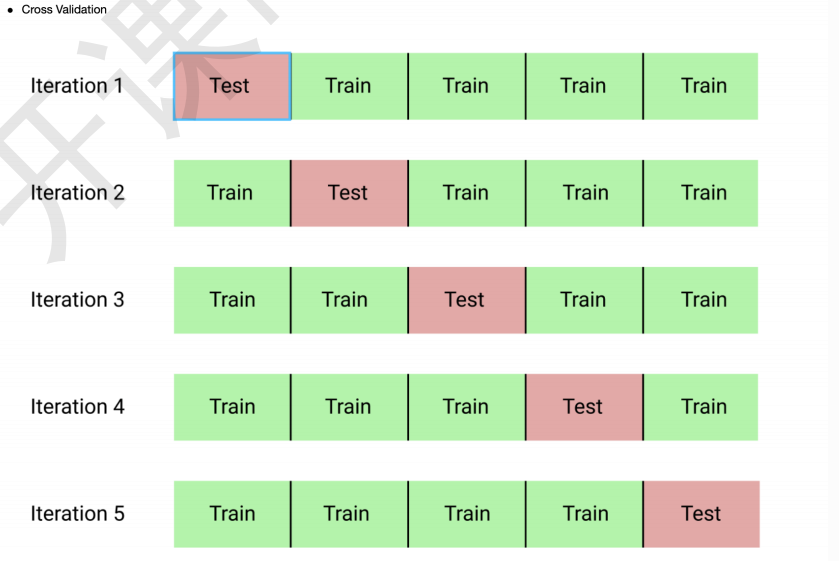
# 得到结果传入DataFrame
results = pd.DataFrame(grid_search.cv_results_)

# 画图操作
figsize(8, 8)
plt.style.use('fivethirtyeight')

plt.plot(results['param_n_estimators'], -1 * results['mean_test_score'], label = 'Testing Error')
plt.plot(results['param_n_estimators'], -1 * results['mean_train_score'], label = 'Training Error')
#横轴是树的个数 ,纵轴是MAE的误差
plt.xlabel('Number of Trees'); plt.ylabel('Mean Abosolute Error'); plt.legend();
plt.title('Performance vs Number of Trees');
#过拟合 , 蓝色平缓 ,红色比较陡 ,中间的数据越来陡,所以overfiting
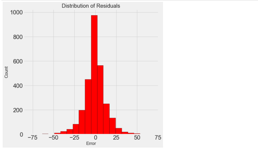
8 评估与测试:预测和真实之间的差异图
# 测试模型
default_model = GradientBoostingRegressor(random_state = 42)
default_model.fit(X,y)
# 选择最好的参数
final_model = grid_search.best_estimator_

final_model
输出:
GradientBoostingRegressor(alpha=0.9, criterion='friedman_mse', init=None,
                          learning_rate=0.1, loss='lad', max_depth=5,
                          max_features=None, max_leaf_nodes=None,
                          min_impurity_decrease=0.0, min_impurity_split=None,
                          min_samples_leaf=6, min_samples_split=6,
                          min_weight_fraction_leaf=0.0, n_estimators=800,
                          n_iter_no_change=None, presort='auto',
                          random_state=42, subsample=1.0, tol=0.0001,
                          validation_fraction=0.1, verbose=0, warm_start=False)
default_pred = default_model.predict(X_test)
final_pred = final_model.predict(X_test)
print('Default model performance on the test set: MAE = %0.4f.' % mae(y_test, default_pred))
print('Final model performance on the test set:   MAE = %0.4f.' % mae(y_test, final_pred))
Default model performance on the test set: MAE = 9.9864.
Final model performance on the test set:   MAE = 9.1172.
Default model performance on the test set: MAE = 9.9864.
Final model performance on the test set:   MAE = 9.1172.

figsize = (6, 6)

# 最终的模型差异 = 模型  -  测试值 ,大部分都在+-25%
residuals = final_pred - y_test

plt.hist(residuals, color = 'red', bins = 20,
         edgecolor = 'black')
plt.xlabel('Error'); plt.ylabel('Count')
plt.title('Distribution of Residuals');

9 解释模型:基于重要性来进行特征选择
import pandas as pd
import numpy as np


pd.options.mode.chained_assignment = None
pd.set_option('display.max_columns', 60)


import matplotlib.pyplot as plt
%matplotlib inline


plt.rcParams['font.size'] = 24

from IPython.core.pylabtools import figsize

import seaborn as sns

sns.set(font_scale = 2)


from sklearn.preprocessing import Imputer, MinMaxScaler

from sklearn.linear_model import LinearRegression
from sklearn.ensemble import GradientBoostingRegressor

from sklearn import tree


import warnings
warnings.filterwarnings("ignore")
- 先拿到我们上个模型的结果
train_features = pd.read_csv('data/training_features.csv')
test_features = pd.read_csv('data/testing_features.csv')
train_labels = pd.read_csv('data/training_labels.csv')
test_labels = pd.read_csv('data/testing_labels.csv')
# 用中值代替缺失值
imputer = Imputer(strategy='median')

# 开始训练
imputer.fit(train_features)


X = imputer.transform(train_features)
X_test = imputer.transform(test_features)


y = np.array(train_labels).reshape((-1,))
y_test = np.array(test_labels).reshape((-1,))
def mae(y_true, y_pred):
    return np.mean(abs(y_true - y_pred))
model = GradientBoostingRegressor(loss='lad', max_depth=5, max_features=None,
                                  min_samples_leaf=6, min_samples_split=6,
                                  n_estimators=800, random_state=42)

model.fit(X, y)
输出:
GradientBoostingRegressor(alpha=0.9, criterion='friedman_mse', init=None,
                          learning_rate=0.1, loss='lad', max_depth=5,
                          max_features=None, max_leaf_nodes=None,
                          min_impurity_decrease=0.0, min_impurity_split=None,
                          min_samples_leaf=6, min_samples_split=6,
                          min_weight_fraction_leaf=0.0, n_estimators=800,
                          n_iter_no_change=None, presort='auto',
                          random_state=42, subsample=1.0, tol=0.0001,
                          validation_fraction=0.1, verbose=0, warm_start=False)
#  GBDT模型作为最终的模型
model_pred = model.predict(X_test)

print('Final Model Performance on the test set: MAE = %0.4f' % mae(y_test, model_pred))
Final Model Performance on the test set: MAE = 9.1485
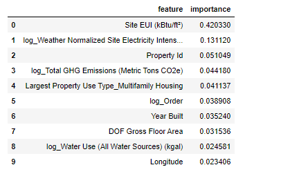
# 特征重要度
feature_results = pd.DataFrame({'feature': list(train_features.columns),  #所有的训练特征
                                'importance': model.feature_importances_})

# 展示前10名的重要的特征 ,降序
feature_results = feature_results.sort_values('importance', ascending = False).reset_index(drop=True)

feature_results.head(10)
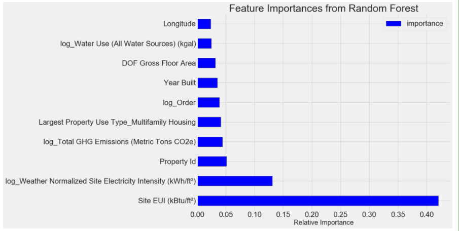
figsize(12, 10)
plt.style.use('fivethirtyeight')

# 展示前10名的重要的特征
feature_results.loc[:9, :].plot(x = 'feature', y = 'importance',
                                 edgecolor = 'k',
                                 kind='barh', color = 'blue');#barh:直方图横着
plt.xlabel('Relative Importance', size = 20); plt.ylabel('')
plt.title('Feature Importances from Random Forest', size = 30);
most_important_features = feature_results['feature'][:10]#前10行的特征
# indices=10个列名
indices = [list(train_features.columns).index(x) for x in most_important_features]# 列表推导式


X_reduced = X[:, indices]
X_test_reduced = X_test[:, indices]

print('Most important training features shape: ', X_reduced.shape)
print('Most important testing  features shape: ', X_test_reduced.shape)
Most important training features shape:  (6622, 10)
Most important testing  features shape:  (2839, 10)
lr = LinearRegression()


lr.fit(X, y)
lr_full_pred = lr.predict(X_test)


lr.fit(X_reduced, y)
lr_reduced_pred = lr.predict(X_test_reduced)


print('Linear Regression Full Results: MAE =    %0.4f.' % mae(y_test, lr_full_pred))
print('Linear Regression Reduced Results: MAE = %0.4f.' % mae(y_test, lr_reduced_pred))
Linear Regression Full Results: MAE =    12.9817.
Linear Regression Reduced Results: MAE = 14.4826.