【机器学习】回归分析、过拟合、分类

一、Linear Regression

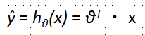
线性回归是相对简单的一种，表达式如下

其中，θ0表示bias，其他可以看做weight，可以转换为如下形式

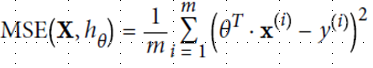
为了更好回归，定义损失函数，并尽量缩小这个函数值，使用MSE方法（mean square equal）

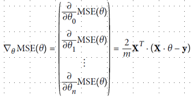
缩小方法采用梯度下降法，即不断地向现在站立的山坡往下走，走的速度就是学习速率η（learning rate），太小耗尽计算资源，太大走过了山谷。

（1）Normal Equation

from sklearn.linear_model import LinearRegression
import numpy as np
import matplotlib.pyplot as plt

# 数据集
X = 2*np.random.rand(100, 1)
y = 4+3*X+np.random.randn(100,1)

# X每个元素加1
X_b = np.c_[np.ones((100,1)), X]
theta_best = np.linalg.inv(X_b.T.dot(X_b)).dot(X_b.T).dot(y)

# 训练
lin_reg = LinearRegression()
lin_reg.fit(X, y)
print(lin_reg.intercept_, lin_reg.coef_)

# 测试数据
X_new = np.array([[0],[2]])
X_new_b = np.c_[np.ones((2,1)), X_new]
y_predict = X_new_b.dot(theta_best)
print(y_predict)

# 画图
plt.plot(X_new, y_predict, "r-")
plt.plot(X, y, "b.")
plt.axis([0,2,0,15])
plt.show()

（2）Batch Gradient Descent

　　基本算是遍历了所有数据，不适用于数据规模大的数据

# BGD梯度下降
eta = 0.1
n_iterations = 1000
m = 100
theta = np.random.randn(2,1)
for iteration in range(n_iterations):
    gradients = 2/m * X_b.T.dot(X_b.dot(theta) - y)
    theta = theta - eta*gradients
print(theta)

可以看出，结果是差不多的

（3）Stochastic Gradient Descent

　　可以避免局部最优结果，但是会震来震去。为了防止这种震荡，让学习速率η不断减小（类似模拟退火）

# SGD梯度下降
m = 100
n_epochs = 50
t0, t1 = 5, 50 # η初始值0.1
def learning_schedule(t):
    return t0 / (t + t1)

theta = np.random.randn(2,1) # random initialization
for epoch in range(n_epochs):
    for i in range(m):
        random_index = np.random.randint(m)
        xi = X_b[random_index:random_index+1]
        yi = y[random_index:random_index+1]
        gradients = 2 * xi.T.dot(xi.dot(theta) - yi)
        eta = learning_schedule(epoch * m + i)
        theta = theta - eta * gradients
print(theta)

# sklearn 提供了SGDRegressor的方法
from sklearn.linear_model import SGDRegressor
sgd_reg = SGDRegressor(max_iter=50, penalty=None, eta0=0.1)
sgd_reg.fit(X, y.ravel())
print(sgd_reg.intercept_, sgd_reg.coef_)

（4）Min-batch Gradient Descent

　　使用小批随机数据，结合SGD与BGD优点

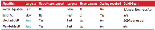
以下是各种方法对比

二、Polynomial Regression

但有的时候，y本身是由x取平方所得，无法找出来一条合适的线性回归线来拟合数据，该怎么办呢？

我们可以尝试将x取平方，取3次方等方法，多加尝试

三、误差分析

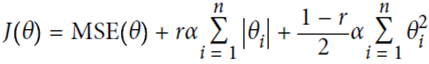
四、防止过拟合

用惩罚系数（penalty），即正则项（regularize the model）

（1）岭回归ridge regression

　　控制参数自由度，减少模型复杂度。所控制的α=α，越大控制结果越强

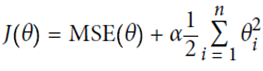
　优势：直接用公式可以计算出结果

from sklearn.linear_model import Ridge
ridge_reg = Ridge(alpha=1, solver="cholesky")
ridge_reg.fit(X, y)

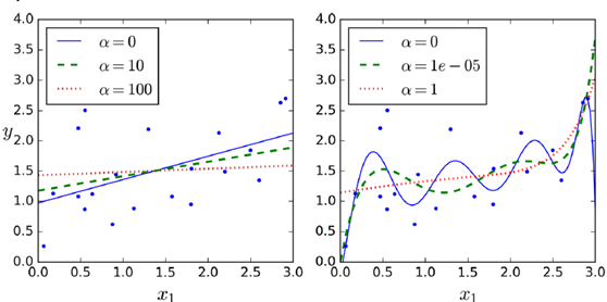
(2)Lasso Regression（least absolute shrinkage and selection operator regression）

正则化项同ridge regression不同，正则化的控制更强

 

# Lasso Regression
from sklearn.linear_model import Lasso
lasso_reg = Lasso(alpha=0.1)
lasso_reg.fit(X, y)
lasso_reg.predict([[1.5]])

对于高阶degree regularize尤为明显，是一个sparse model，很多高阶参数项成为了0

 （3）Elastic Net（一般推荐使用）

 相当于ridge和lasso regression的结合，用超参数r来控制其平衡

# Elastic Net
from sklearn.linear_model import ElasticNet
elastic_net = ElasticNet(alpha=0.1, l1_ratio=0.5)
elastic_net.fit(X, y)

（4）Early Stopping

找到开始上升的点，从那里停止（整体找到，取最优的）

from sklearn.base import clone
sgd_reg = SGDRegressor(n_iter=1, warm_start=True, penalty=None,
                                             learning_rate="constant", eta0=0.0005)
minimum_val_error = float("inf")
best_epoch = None
best_model = None
for epoch in range(1000):
    sgd_reg.fit(X_train_poly_scaled, y_train) # continues where it left off
    y_val_predict = sgd_reg.predict(X_val_poly_scaled)
    val_error = mean_squared_error(y_val_predict, y_val)
    if val_error < minimum_val_error:
        minimum_val_error = val_error
        best_epoch = epoch
        best_model = clone(sgd_reg)

五、Logistic Regression（可用作分类）

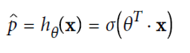
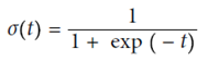（使用sigmod函数，y在（0,1）之间）

定义cost function，由于p在（0,1）之间，故最前面加一个符号，保证代价始终为正的。p值越大，整体cost越小，预测的越对

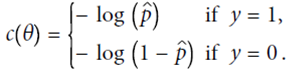
即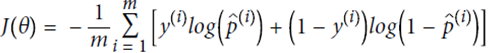

不存在解析解，故用偏导数计算

以Iris花的种类划分为例

import matplotlib.pyplot as plt
from sklearn import datasets
iris = datasets.load_iris()
print(list(iris.keys()))
# ['DESCR', 'data', 'target', 'target_names', 'feature_names']
X = iris["data"][:, 3:] # petal width
y = (iris["target"] == 2).astype(np.int) # 1 if Iris-Virginica, else 0

from sklearn.linear_model import LogisticRegression
log_reg = LogisticRegression()
log_reg.fit(X, y)
X_new = np.linspace(0, 3, 1000).reshape(-1, 1)
# estimated probabilities for flowers with petal widths varying from 0 to 3 cm:
y_proba = log_reg.predict_proba(X_new)

plt.plot(X_new, y_proba[:, 1], "g-", label="Iris-Virginica")
plt.plot(X_new, y_proba[:, 0], "b--", label="Not Iris-Virginica")
plt.show()
# + more Matplotlib code to make the image look pretty

六、Softmax Regression

可以用做多分类

使用交叉熵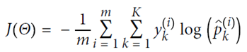

　　

X = iris["data"][:, (2, 3)] # petal length, petal width
y = iris["target"]
softmax_reg = LogisticRegression(multi_class="multinomial",solver="lbfgs", C=10)
softmax_reg.fit(X, y)

print(softmax_reg.predict([[5, 2]]))
# array([2])
print(softmax_reg.predict_proba([[5, 2]]))
# array([[ 6.33134078e-07, 5.75276067e-02, 9.42471760e-01]])