图形预览:

0、import
import numpy as np
from matplotlib import pyplot as plt
from mpl_toolkits.mplot3d import Axes3D
1、开口向上的抛物面
fig = plt.figure(figsize=(9,6),
                 facecolor='khaki'
                )
ax = fig.gca(projection='3d')

# 二元函数定义域平面集
x = np.linspace(start=-3,
                stop=3,
                num=100
               )
y = np.linspace(start=-3,
                stop=3,
                num=100
               )
X, Y = np.meshgrid(x, y)    # 网格数据
Z = np.power(X, 2) + np.power(Y, 2)    # 二元函数 z = x**2 + y**2

# 绘图
surf = ax.plot_surface(X=X,
                       Y=Y,
                       Z=Z,
                       rstride=2,    # row stride, 行跨度
                       cstride=2,    # column stride, 列跨度
                       color='r',
                       linewidth=0.5,
                      )

# 调整视角
ax.view_init(elev=7,    # 仰角
             azim=30   # 方位角
            )

# 显示图形
plt.show()
图形:

2、开口向下的抛物面
fig = plt.figure(figsize=(9,6),
                 facecolor='khaki'
                )
ax = fig.gca(projection='3d')

# 二元函数定义域平面集
x = np.linspace(start=-3,
                stop=3,
                num=100
               )
y = np.linspace(start=-3,
                stop=3,
                num=100
               )
X, Y = np.meshgrid(x, y)    # 网格数据
Z = np.power(X, 2) + np.power(Y, 2)    # 二元函数 z = x**2 + y**2

# 绘图
surf = ax.plot_surface(X=X,
                       Y=Y,
                       Z=-Z,
                       rstride=2,    # row stride, 行跨度
                       cstride=2,    # column stride, 列跨度
                       color='g',
                       linewidth=0.5,
                      )

# 调整视角
ax.view_init(elev=7,    # 仰角
             azim=30   # 方位角
            )

# 显示图形
plt.show()
图形:

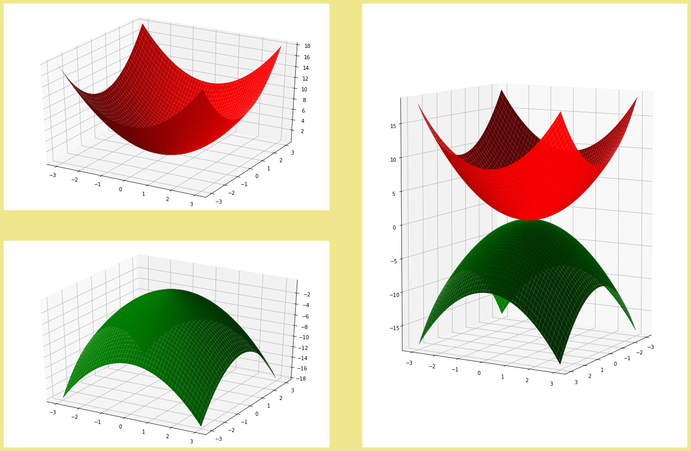
3、用多子区显示不同抛物面
fig = plt.figure(figsize=(24, 16),
                 facecolor='khaki'
                )

# 二元函数定义域平面集
x = np.linspace(start=-3,
                stop=3,
                num=100
               )
y = np.linspace(start=-3,
                stop=3,
                num=100
               )
X, Y = np.meshgrid(x, y)    # 网格数据
Z = np.power(X, 2) + np.power(Y, 2)    # 二元函数 z = x**2 + y**2

# -------------------------------- subplot(221) --------------------------------
ax = fig.add_subplot(221, projection='3d')

# 开口向上的抛物面
surf = ax.plot_surface(X=X,
                       Y=Y,
                       Z=Z,
                       rstride=2,    # row stride, 行跨度
                       cstride=2,    # column stride, 列跨度
                       color='r',
                       linewidth=0.5,
                      )

# -------------------------------- subplot(223) --------------------------------
ax = fig.add_subplot(223, projection='3d')

# 开口向下的抛物面
surf = ax.plot_surface(X=X,
                       Y=Y,
                       Z=-Z,
                       rstride=2,    # row stride, 行跨度
                       cstride=2,    # column stride, 列跨度
                       color='g',
                       linewidth=0.5,
                      )

# -------------------------------- subplot(22, (2,4)) --------------------------------
ax = plt.subplot2grid(shape=(2,2),
                      loc=(0, 1),
                      rowspan=2,
                      projection='3d'
                     )

# 开口向上的抛物面
surf1 = ax.plot_surface(X=X,
                        Y=Y,
                        Z=Z,
                        rstride=2,    # row stride, 行跨度
                        cstride=2,    # column stride, 列跨度
                        color='r',
                        linewidth=0.5,
                       )
# 开口向下的抛物面
surf2 = ax.plot_surface(X=X,
                        Y=Y,
                        Z=-Z,
                        rstride=2,    # row stride, 行跨度
                        cstride=2,    # column stride, 列跨度
                        color='g',
                        linewidth=0.5,
                      )

# 调整视角
ax.view_init(elev=7,    # 仰角
             azim=30   # 方位角
            )

# -------------------------------- fig --------------------------------
# 调整子区布局
fig.subplots_adjust(wspace=0.1,    # width space
                    hspace=0.15    # height space
                   )

# 显示图形
plt.show()
图形:
软件版本: